Chromeでデベロッパーツールを開くとwasmが遅くなる現象
概要
Rustでwasm生成する練習のため、実践Rustプログラミング入門を参考にしてマンデルブロ集合の計算のwasmとjsで速度比較するWebページを作成しました。
- 作成したWebページ:https://taketakeyyy.github.io/tools/wasm-vs-js-mandelbrot/wasm-vs-js-mandelbrot.html
- ソースコード:https://github.com/taketakeyyy/wasm-vs-js-mandlbrot
しかし開発中、wasmの速度が遅くなったり速くなったりする挙動に悩まされました。色々調べた結果、Chromeでデベロッパーツールを開いているか否かが原因だったようです。
比較
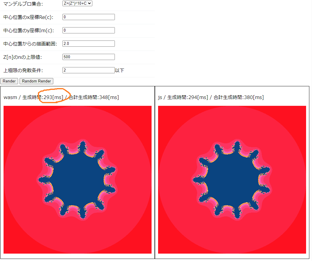
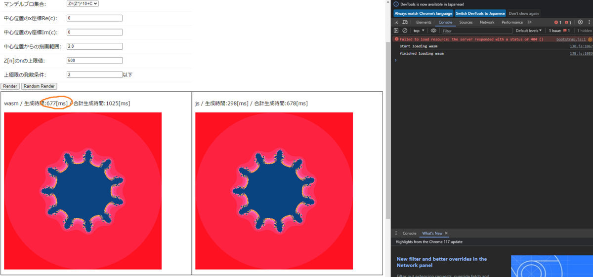
なんでこうなるのか全くわかっていません🤷後述追記した。
この現象はlocalhostや本番環境関係なく発生しています。
デベロッパツールを開いてconsole.logで時間計測する際には注意が必要になりそうです。
「wasm 遅い」で検索すると色々出てきますが、こういうのも原因のひとつになっているんじゃないかと思いました。
2023/09/21 0:56 追記
Twitter(X)でご指摘いただきました。ありがとうございます。
Chrome において、DevTools をただ開くと wasm の実行が極めて遅くなる現象が確認されております。これはバグではなくて仕様なのですが、結構複雑な仕様で、
DevTools を開くと TurboFan の最適化がキャンセルされて遅くなる しかし Profile タブで Profile を取るときには再度 TurboFan の最適化が適用される という挙動になっております。Chrome では、ただ DevTools を開いているだけで wasm の実行がかなり遅くなります。大変気づきにくいトリガーなので、wasm 系の開発をされる時にはお気をつけください。
そういう仕様らしいです。
その他
- localhost の WebAssembly は遅いので気を付けろ! - Qiita
- 最初これかなと思ったけど、関係なかった
- ブラウザによっても速度は変わる(これはそういうもの)
- Firefox:117.0.1 (64 ビット)で試したらwasmが明らかに遅かった
2人の子供問題のパラドックスを利用したギャンブル
前提条件
A「ある家庭に2人の子供がいて、1人が男の子の場合、もう1人の子が女の子である確率は?」
B「ある家庭で男の子が生まれる確率と女の子が生まれる確率はそれぞれ1/2ずつで考えていい?」
A「いいよ」
B「うーん。もう1人の子が男の子か女の子かは独立だから、1/2じゃない?」
A「残念。ある家庭に2人の子供がいる場合の(年上, 年下)のペアは(男, 男)、(男, 女)、(女, 男)、(女, 女)の4通りで、1人が男の子で確定したときに(女, 女)は除外される。だから残りの3通りのうち、もう1人が女の子のパターンは(男, 女)、(女, 男)の2通りだから答えは2/3だよ」
B「なるほどなぁ」
ギャンブルに持ち込む
A「よし、今の2人の子供の問題と同じ状況を再現して賭けをしようよ」
B「どんな賭け?」
A「僕は2枚のコインを同時に投げる。1枚のコインはみんなに見えるように。もう1枚のコインは表か裏どちらが出たのか僕も君もわからないようにする。」
B「それで?」
A「見えてるコインが表になったときに賭けは始まるんだ。『見えてないコインが裏であるか賭けてください』って。裏だったら君の勝ち。そうじゃなかったら僕の勝ちだ。さっきの2人の子供と同じ状況だから、見えてないコインが裏の確率は2/3だよね?」
B「そうかも」
A「見えてるコインが裏になったときはコインを投げ直すよ」
B「まあいいでしょう」
A「当たったときの賞金は僕が1000円出す。当たる確率が2/3だから賞金の期待値は666円だね。参加費は1回600円でどう?これは君にバチクソ有利な賭けだよ」
B「やろうやろう」
# coding: utf-8
import random

entry_fee = 600 # 参加費
prize = 1000 # 賞金
bet_num = 0 # 賭けを行った回数
iter_max = 1000 # コインを投げた回数
win_b = 0 # B君が勝った回数

for i in range(iter_max):
    seen = random.randrange(2) # 見えているコイン(0:表, 1:裏)
    unseen = random.randrange(2) # 見えてないコイン(0:表, 1:裏)
    if seen==0:
        # 見えてるコインが表になったら賭けをする
        bet_num += 1
        if unseen==1:
            # 見えてないコインが裏だった場合、B君の勝ち
            win_b += 1

print("賭けを行った回数: {}".format(bet_num))
print("B君の勝率: {}".format(win_b/bet_num))
print("B君が払った参加費の合計: {}".format(entry_fee*bet_num))
print("B君が貰った賞金の合計: {}".format(prize*win_b))
print("B君の収支: {}".format(prize*win_b - entry_fee*bet_num))
賭けを行った回数: 524
B君の勝率: 0.5305343511450382
B君が払った参加費の合計: 314400
B君が貰った賞金の合計: 278000
B君の収支: -36400
1時間後
B「3万円も負けちゃった」
A「そういうときもあるよ」
B「わかった。見えてるコインが裏になったときにコインを投げ直しているのがイカサマだ。試行をごまかそうとしたね?」
A「じゃあ見えているコインが裏になったときも賭けをしよう。そのときは『見えてないコインが表であるか賭けてください』だね。表だったら君の勝ち。そうじゃなかったら僕の勝ちだ。これは見えているコインが表のときと同じ賭けだから問題ないよね?」
B「それならいいかも」
A「じゃあ続けるよ」
# coding: utf-8
import random

entry_fee = 600 # 参加費
prize = 1000 # 賞金
bet_num = 0 # 賭けを行った回数
iter_max = 1000 # コインを投げた回数
win_b = 0 # B君が勝った回数

for i in range(iter_max):
    seen = random.randrange(2) # 見えているコイン(0:表, 1:裏)
    unseen = random.randrange(2) # 見えてないコイン(0:表, 1:裏)
    if seen==0:
        # 見えてるコインが表になったら賭けをする
        bet_num += 1
        if unseen==1:
            # 見えてないコインが裏だった場合、B君の勝ち
            win_b += 1
    # 【追加】
    elif seen==1:
        # 見えてるコインが裏になったときも賭けをする
        bet_num += 1
        if unseen==0:
            # 見えてないコインが表だった場合、B君の勝ち
            win_b += 1

print("賭けを行った回数: {}".format(bet_num))
print("B君の勝率: {}".format(win_b/bet_num))
print("B君が払った参加費の合計: {}".format(entry_fee*bet_num))
print("B君が貰った賞金の合計: {}".format(prize*win_b))
print("B君の収支: {}".format(prize*win_b - entry_fee*bet_num))
賭けを行った回数: 1000
B君の勝率: 0.512
B君が払った参加費の合計: 600000
B君が貰った賞金の合計: 512000
B君の収支: -88000
さらに1時間後
B「なるほど、ひとつだけわかったことがある」
A「それはなに?」
B「君との友情はもう壊れたってこと」
A「😅トホホ・・・」
解説
- 2人の子供問題のパラドックスの本質は、「確率は1/2ではなく、実は確率は2/3でした」というより、「問題文が曖昧なので1/2と解釈することも2/3と解釈することもできる」点にあるだろう
- その曖昧さを利用して、相手に「実は確率は2/3」であることを納得させる
- あとは似て非なる「本当の確率は1/2」のギャンブルに持ち込み、ボロ儲けする
B君がやるべきだったギャンブル
# coding: utf-8
import random

entry_fee = 600 # 参加費
prize = 1000 # 賞金
bet_num = 0 # 賭けを行った回数
iter_max = 1000 # 家庭を訪問する回数
win = 0 # B君が勝った回数

for i in range(iter_max):
    pair = random.randrange(4) # ある家庭の2人の子供の(年上,年下)のペア: 0:(男,男),1:(男,女),2:(女,男),3:(女,女)
    if pair!=3:
        # 少なくとも1人が男と判明した場合、賭けが始まる
        bet_num += 1
        if pair!=0:
            # (男,女),(女,男)の場合は、B君の勝ち
            win += 1

print("賭けを行った回数: {}".format(bet_num))
print("B君の勝率: {}".format(win/bet_num))
print("B君が払った参加費の合計: {}".format(entry_fee*bet_num))
print("B君が貰った賞金の合計: {}".format(prize*win))
print("B君の収支: {}".format(prize*win - entry_fee*bet_num))
賭けを行った回数: 748
B君の勝率: 0.6644385026737968
B君が払った参加費の合計: 448800
B君が貰った賞金の合計: 497000
B君の収支: 48200
Qiskit Global Summer School 2023 Lab5 参加記録
各Labの記録
- 参加結果の記事:Qiskit Global Summer School 2023 参加記録
- Lab1:記事なし。かなり基礎的な内容だった気がするので
- Lab2:Qiskit Global Summer School 2023 Lab2 参加記録
- Lab3:Qiskit Global Summer School 2023 Lab3 参加記録
- Lab4:Qiskit Global Summer School 2023 Lab4 参加記録
- Lab5:Qiskit Global Summer School 2023 Lab5 参加記録
まえがき
Qiskit Global Summer School 2023 Lab5の記録です。
Lab 5: Error mitigation with Qiskit Runtime
- エラー緩和(Error mitigation)をするラボ。
- 具体的には、単純な観測値と初期状態を定義し、Estimatorプリミティブを使って期待値を測定する。
- ノイズの多いシミュレーションを用いて、さまざまなエラー緩和戦略の効果を探る。
Setup
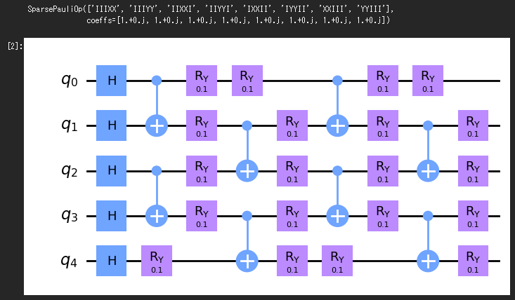
例として簡単なハイゼンベルグ・ハミルトニアン・モデルを定義する。また、簡単な状態準備回路を構築する。
from qiskit import QuantumCircuit, QuantumRegister
from qiskit.quantum_info import SparsePauliOp


def heisenberg_hamiltonian(
    length: int, jx: float = 1.0, jy: float = 0.0, jz: float = 0.0
) -> SparsePauliOp:
    terms = []
    for i in range(length - 1):
        if jx:
            terms.append(("XX", [i, i + 1], jx))
        if jy:
            terms.append(("YY", [i, i + 1], jy))
        if jz:
            terms.append(("ZZ", [i, i + 1], jz))
    return SparsePauliOp.from_sparse_list(terms, num_qubits=length)


def state_prep_circuit(num_qubits: int, layers: int = 1) -> QuantumCircuit:
    qubits = QuantumRegister(num_qubits, name="q")
    circuit = QuantumCircuit(qubits)
    circuit.h(qubits)
    for _ in range(layers):
        for i in range(0, num_qubits - 1, 2):
            circuit.cx(qubits[i], qubits[i + 1])
        circuit.ry(0.1, qubits)
        for i in range(1, num_qubits - 1, 2):
            circuit.cx(qubits[i], qubits[i + 1])
        circuit.ry(0.1, qubits)
    return circuit
length = 5

hamiltonian = heisenberg_hamiltonian(length, 1.0, 1.0)
circuit = state_prep_circuit(length, layers=2)

print(hamiltonian)
circuit.draw("mpl")
Calculate exact expectation value (energy)(翻訳)
まず、Estimatorプリミティブのローカルシミュレータ実装を使って正確な期待値を計算する。ハミルトニアンの期待値は "エネルギー "とも呼ばれる。
from qiskit_aer.primitives import Estimator

estimator = Estimator(approximation=True)
job = estimator.run(circuit, hamiltonian, shots=None)
result = job.result()
exact_value = result.values[0]

print(f"Exact energy: {exact_value}")
# Exact energy: 4.290938711029713
Run noisy simulation through Qiskit Runtime
次に、Qiskit Runtimeサービスを初期化し、ノイズを扱えるシミュレータに支えられたEstimatorプリミティブの使用に切り替える。この回路は5量子ビットで動作するが、量子ビット選択の潜在的な効果を後で示すために、6量子ビットでシミュレータを初期化する。
from qiskit_ibm_runtime import QiskitRuntimeService

hub = "ibm-q-internal" # この辺の値は適宜自分用に変える
group = "deployed" #
project = "default" #

service = QiskitRuntimeService(instance=f"{hub}/{group}/{project}")
from qiskit_ibm_runtime import Estimator, Options, Session
from qiskit.transpiler import CouplingMap

backend = service.get_backend("simulator_statevector")
# set simulation options
simulator = {
    "basis_gates": ["id", "rz", "sx", "cx", "reset"],
    "coupling_map": list(CouplingMap.from_line(length + 1)),
}
shots = 10000
No noise
まずはノイズなしのシミュレータで実行してみる。
from qiskit_ibm_runtime import Estimator, Options, Session
from qiskit.transpiler import CouplingMap
import math

options = Options(
    simulator=simulator,
    resilience_level=0,
)

with Session(service=service, backend=backend):
    estimator = Estimator(options=options)
    job = estimator.run(circuit, hamiltonian, shots=shots)

result = job.result()
experiment_value = result.values[0]
error = abs(experiment_value - exact_value)
variance = result.metadata[0]["variance"]
std = math.sqrt(variance / shots)

print(f"Estimated energy: {experiment_value}")
print(f"Energy error: {error}")
print(f"Variance: {variance}")
print(f"Standard error: {std}")
Estimated energy: 4.275399999999999
Energy error: 0.015538711029713603
Variance: 4.44106724
Standard error: 0.021073839801991474
誤差(Energy error)が 0.015... という値になった。ノイズなしでこのくらいになると覚えておいて、以下を進めていこう。
Readout error
次に、Readout error(読み出しエラー)ありのシミュレータで実行してみる。
ex1
この課題では、本当に悪い Readout error を持つ最初の量子ビットを除いたすべての量子ビットのReadout errorが緩やかなノイズモデルを構築する。
具体的には、以下の特性を持つノイズモデルを構築すること:
- q0
- 50%の確率で1を0と読み間違える
- 20%の確率で0を1と読み間違える
- それ以外の量子ビット
- 5%の確率で1を0と読み間違える
- 2%の確率で0を1と読み間違える
ノイズ作るライブラリは以下たちを参照すると良い。
- https://qiskit.org/ecosystem/aer/apidocs/aer_noise.html
- https://qiskit.org/ecosystem/aer/tutorials/3_building_noise_models.html
from qiskit_aer.noise import NoiseModel, ReadoutError

noise_model = NoiseModel()

##### your code here #####
# その他の量子ビットに与えるReadoutError
rest_p0given1 = 0.05 # P(0|1)
rest_p1given0 = 0.02 # P(1|0)
# ReadoutErrorには [[P(0|0), P(1|0)], [P(0|1), P(1|1)]] のフォーマットで与える
rest_readout_error = ReadoutError([[1 - rest_p1given0, rest_p1given0], [rest_p0given1, 1 - rest_p0given1]])
noise_model.add_all_qubit_readout_error(rest_readout_error)

# q0に与えるReadoutError
q0_p0given1 = 0.5
q0_p1given0 = 0.2
q0_readout_error = ReadoutError([[1 - q0_p1given0, q0_p1given0], [q0_p0given1, 1 - q0_p0given1]])
noise_model.add_readout_error(q0_readout_error, (0,))

print(noise_model)
WARNING: Specific readout error on qubits (0,) overrides previously defined all-qubit readout error for these qubits.
NoiseModel:
  Basis gates: ['cx', 'id', 'rz', 'sx']
  Instructions with noise: ['measure']
  Qubits with noise: [0]
  All-qubits errors: ['measure']
  Specific qubit errors: [('measure', (0,))]
まず、読み出しエラーを緩和するために何もせずにシミュレーションを実行してみる。明示的にresilience_level = 0を設定し、Runtimeサービスによるエラー緩和が適用されないようにする。不適切な量子ビットの選択の影響を説明するために、量子ビット0を含む初期レイアウトを明示的に指定する。
options = Options(
    simulator=dict(noise_model=noise_model, **simulator),
    resilience_level=0,
    transpilation=dict(initial_layout=list(range(length))),
)

with Session(service=service, backend=backend):
    estimator = Estimator(options=options)
    job = estimator.run(circuit, hamiltonian, shots=shots)

result = job.result()
experiment_value = result.values[0]
error = abs(experiment_value - exact_value)
variance = result.metadata[0]["variance"]
std = math.sqrt(variance / shots)

print(f"Estimated energy: {experiment_value}")
print(f"Energy error: {error}")
print(f"Variance: {variance}")
print(f"Standard error: {std}")
Estimated energy: 3.5386
Energy error: 0.7523387110297128
Variance: 5.337599239999999
Standard error: 0.023103244880319302
この誤差(Energy error)はかなり大きい。これを改善するために、量子ビット0を避けるような量子ビットレイアウトを選んでみよう。
options = Options(
    simulator=dict(noise_model=noise_model, **simulator),
    resilience_level=0,
    transpilation=dict(initial_layout=list(range(1, length + 1))), # initial_layoutからq0を取り除く
)

with Session(service=service, backend=backend):
    estimator = Estimator(options=options)
    job = estimator.run(circuit, hamiltonian, shots=shots)

result = job.result()
experiment_value = result.values[0]
error = abs(experiment_value - exact_value)
variance = result.metadata[0]["variance"]
std = math.sqrt(variance / shots)

print(f"Estimated energy: {experiment_value}")
print(f"Energy error: {error}")
print(f"Variance: {variance}")
print(f"Standard error: {std}")
Estimated energy: 3.9506
Energy error: 0.3403387110297129
Variance: 4.962461319999999
Standard error: 0.02227658259248936
誤差(Energy error)は小さくなったが、それでもまだ大きい。resilience_level = 1に設定して、読み出しエラー緩和を有効にしてみよう。
options = Options(
    simulator=dict(noise_model=noise_model, **simulator),
    resilience_level=1, # 1に設定
    transpilation=dict(initial_layout=list(range(1, length + 1))),
)

with Session(service=service, backend=backend):
    estimator = Estimator(options=options)
    job = estimator.run(circuit, hamiltonian, shots=shots)

result = job.result()
experiment_value = result.values[0]
error = abs(experiment_value - exact_value)
variance = result.metadata[0]["variance"]
std = math.sqrt(variance / shots)

print(f"Estimated energy: {experiment_value}")
print(f"Energy error: {error}")
print(f"Variance: {variance}")
print(f"Standard error: {std}")
Estimated energy: 4.303468384959293
Energy error: 0.012529673929580376
Variance: 7.169951196036428
Standard error: 0.02677676454696577
誤差(Energy error)はかなり小さくなり、読み出しエラーの影響はほぼ完全に緩和されたことがわかった。この緩和は「タダ」ではない。特に、
- 読み出しエラーを緩和するために、ランタイムサービスは追加のキャリブレーション回路を実行する必要があるため、全体的な実行時間が長くなる可能性がある。
- 推定値の分散が大きくなり、平均値の標準誤差が大きくなる。その結果、所定の標準誤差を達成するためには、より多くのショットを指定する必要がある。
通常このようなコストは比較的小さいため、読み出しエラーの緩和を可能にすることは、ほとんどの場合、価値がある。
ex2
読み出しエラーの緩和をオンにすると、推定値の分散(Variance)が2倍増加すると仮定する。 元々10,000ショットで実験を行った場合、平均の標準誤差(Standard error)を同じにするためには今何ショットを使用すべきか?
元々ショットで実験を行った場合の標準偏差を
とする。
読み出しエラーの緩和をオンにしたときのショット数を、標準偏差を
とする。
読み出しエラーの緩和をオンにすると分散が2倍になるので、標準偏差は倍になる。よって
標準誤差 より、
を解けばいい。 よって
new_shots: int

##### your code here #####
new_shots = 20000
Depolarizing error and zero-noise extrapolation
このセクションでは、ゼロノイズ外挿(zero-noise extrapolation)を使ってどのように脱分極エラー(depolarizing error)を軽減できるかを見ていく。Qiskit Runtimeのゼロノイズ外挿機能はまだベータ版であるため、現在いくつかの制限がある。
特に、本稿執筆時点では、ゼロノイズ外挿機能は読み出しエラーを緩和しない。
したがって以下の例では、ノイズモデルから読み出しエラーを取り除く。
ex3
各CNOTゲートの後に2量子ビットの脱分極エラーを加えるノイズモデルを構築し、エラーチャネルが1%の確率で入力量子状態を完全混合状態にマップするようにする。
depolarizing_error- 第1引数:確率
- 第2引数:n-qubit用の脱分極エラーかを指定する
今回CNOTゲートは2-qubitゲートなので、第2引数は2を指定する。
詳しい使い方はNoise Models (qiskit_aer.noise)の「Example: depolarizing noise model」に書いてある。
from qiskit_aer.noise import depolarizing_error

noise_model = NoiseModel()

##### your code here #####
depolar_p = 0.01
depolar_error = depolarizing_error(depolar_p, 2)

noise_model.add_all_qubit_quantum_error(depolar_error, ['cx']) # CNOTゲートに脱分極エラーを適用

print(noise_model)
NoiseModel:
  Basis gates: ['cx', 'id', 'rz', 'sx']
  Instructions with noise: ['cx']
  All-qubits errors: ['cx']
resilience_level = 0でestimatorを実行してみる。
# resilience_level = 0で実行
options = Options(
    simulator=dict(noise_model=noise_model, **simulator),
    resilience_level=0, # 0で実行
)

with Session(service=service, backend=backend):
    estimator = Estimator(options=options)
    job = estimator.run(circuit, hamiltonian, shots=shots)

result = job.result()
experiment_value = result.values[0]
error = abs(experiment_value - exact_value)
variance = result.metadata[0]["variance"]
std = math.sqrt(variance / shots)

print(f"Estimated energy: {experiment_value}")
print(f"Energy error: {error}")
print(f"Variance: {variance}")
print(f"Standard error: {std}")
Estimated energy: 4.0624
Energy error: 0.2285387110297128
Variance: 4.79633856
Standard error: 0.021900544650761543
次はresilience_level = 1で読み出しエラーの緩和をオンにしてestimatorを実行してみよう。今このノイズモデルには読み出しエラーの緩和は含まれていないため、これによる効果は期待できない。
options = Options(
    simulator=dict(noise_model=noise_model, **simulator),
    resilience_level=1, # 1に設定して読み出しエラーの緩和をオンにする
)

with Session(service=service, backend=backend):
    estimator = Estimator(options=options)
    job = estimator.run(circuit, hamiltonian, shots=shots)

result = job.result()
experiment_value = result.values[0]
error = abs(experiment_value - exact_value)
variance = result.metadata[0]["variance"]
std = math.sqrt(variance / shots)

print(f"Estimated energy: {experiment_value}")
print(f"Energy error: {error}")
print(f"Variance: {variance}")
print(f"Standard error: {std}")
Estimated energy: 4.0586
Energy error: 0.23233871102971282
Variance: 4.8106246
Standard error: 0.02193313611866757
予想通り、resilience_level = 0のときと誤差(Energy error)は変わらない結果となった。
では、resilience_level = 2に設定して、ゼロノイズ外挿をオンにして実行してみよう。
options = Options(
    simulator=dict(noise_model=noise_model, **simulator),
    resilience_level=2, # 2に設定してゼロノイズ外挿をオンにする
)

with Session(service=service, backend=backend):
    estimator = Estimator(options=options)
    job = estimator.run(circuit, hamiltonian, shots=shots)

result = job.result()
experiment_value = result.values[0]
error = abs(experiment_value - exact_value)
variances = result.metadata[0]["zne"]["noise_amplification"]["variance"]
std = [math.sqrt(var/shots) for var in variances]

print(f"Estimated energy: {experiment_value}")
print(f"Energy error: {error}")
print(f"Variances: {variances}")
print(f"Standard error: {std}")
Estimated energy: 4.206533333333335
Energy error: 0.08440537769637846
Variances: [4.84564196, 5.46333092, 5.91612628]
Standard error: [0.022012818901721787, 0.02337376931519604, 0.024323088372984216]
誤差(Energy error)がかなり小さくなったことがわかる。脱分極ノイズの影響はほぼ完全に緩和されたおかげである。
推定量に対する単一の分散値を得る代わりに、外挿のために測定された各データポイントに対する分散のリストを返すようになったことに注意。Qiskit Runtimeの将来のバージョンでは、これらの分散も外挿され、最終的な推定量に対して単一の分散が返されるようになるだろう。
ex4(ungraded)
脱分極エラー(depolarizing error)以外に、どのような種類のノイズがゼロノイズ外挿によって緩和できるだろうか?他のノイズモデルを構築し、ゼロノイズ外挿を使った場合と使わない場合でシミュレーションを行い、あなたの提案をテストしてみよ。
Noise Models (qiskit_aer.noise) の「Quantum Error Functions」の項目に色々エラーの種類が書いてある。
以下の記事を大いに参考にした。
Coherent Noiseをrx,ry,rzゲートに使ってみる。
# Coherent Noise
from qiskit_aer.noise import coherent_unitary_error
from qiskit.circuit.library import RYGate, RXGate, RZGate

noise_model = NoiseModel()

epsilon = math.pi/30 # over rotation amount

# RYゲートのコヒーレントノイズ
epsilon_rotation = RYGate(epsilon).to_matrix() # get matrix representation
over_rotation = coherent_unitary_error(epsilon_rotation)
# for i in range(5):
#     noise_model.add_quantum_error(over_rotation, ['ry'], qubits=[i])
noise_model.add_all_qubit_quantum_error(over_rotation, ['ry'])

# RXゲートのコヒーレントノイズ
epsilon_rotation = RXGate(epsilon).to_matrix()
over_rotation = coherent_unitary_error(epsilon_rotation)
noise_model.add_all_qubit_quantum_error(over_rotation, ['rx'])

# RZゲートのコヒーレントノイズ
epsilon_rotation = RZGate(epsilon).to_matrix()
over_rotation = coherent_unitary_error(epsilon_rotation)
noise_model.add_all_qubit_quantum_error(over_rotation, ['rz'])

print(noise_model)
NoiseModel:
  Basis gates: ['cx', 'id', 'rx', 'ry', 'rz', 'sx']
  Instructions with noise: ['ry', 'rx', 'rz']
  All-qubits errors: ['ry', 'rx', 'rz']
まずはresilience_level = 0で実行。
options = Options(
    simulator=dict(noise_model=noise_model, **simulator),
    resilience_level=0, # resilience_level = 0で実行
)

with Session(service=service, backend=backend):
    estimator = Estimator(options=options)
    job = estimator.run(circuit, hamiltonian, shots=shots)

result = job.result()
experiment_value = result.values[0]
error = abs(experiment_value - exact_value)
variance = result.metadata[0]["variance"]
std = math.sqrt(variance / shots)

print(f"Estimated energy: {experiment_value}")
print(f"Energy error: {error}")
print(f"Variance: {variance}")
print(f"Standard error: {std}")
Estimated energy: 3.9776
Energy error: 0.3133387110297132
Variance: 4.8817328
Standard error: 0.02209464369479626
次にresilience_level = 2で実行。
options = Options(
    simulator=dict(noise_model=noise_model, **simulator),
    resilience_level=2, # resilience_level = 2で実行
)

with Session(service=service, backend=backend):
    estimator = Estimator(options=options)
    job = estimator.run(circuit, hamiltonian, shots=shots)

result = job.result()
experiment_value = result.values[0]
error = abs(experiment_value - exact_value)
variances = result.metadata[0]["zne"]["noise_amplification"]["variance"]
std = [math.sqrt(var/shots) for var in variances]

print(f"Estimated energy: {experiment_value}")
print(f"Energy error: {error}")
print(f"Variances: {variances}")
print(f"Standard error: {std}")
Estimated energy: 3.6169500000000014
Energy error: 0.6739887110297116
Variances: [5.236187, 5.256725159999999, 5.26025432]
Standard error: [0.022882716184928747, 0.02292754928028724, 0.02293524431960558]
ゼロノイズ外挿によって緩和しなかった。というか誤差(Energy error)がひどくなってる。
pauli_errorをid,rx,ry,rzゲートに使ってみる
ある確率でbit-flipエラーやphase-flipエラーを起こすノイズを追加する。
from qiskit_aer.noise import pauli_error

# Construct a 1-qubit bit-flip and phase-flip errors
p_error = 0.01

# 確率p_errorでXゲートが適用される。確率1-p_errorでIゲートが適用される(何もしない)
bit_flip_error = pauli_error([('X', p_error), ('I', 1 - p_error)])
# 確率p_errorでZゲートが適用される。確率1-p_errorでIゲートが適用される(何もしない)
phase_flip_error = pauli_error([('Z', p_error), ('I', 1 - p_error)])

noise_model = NoiseModel()

noise_model.add_all_qubit_quantum_error(bit_flip_error, ['id', "rx", "ry", "rz"])
noise_model.add_all_qubit_quantum_error(phase_flip_error, ['id', "rx", "ry", "rz"])

print(noise_model)
WARNING: all-qubit error already exists for instruction "id", composing with additional error.
WARNING: all-qubit error already exists for instruction "rx", composing with additional error.
WARNING: all-qubit error already exists for instruction "ry", composing with additional error.
WARNING: all-qubit error already exists for instruction "rz", composing with additional error.
NoiseModel:
  Basis gates: ['cx', 'id', 'rx', 'ry', 'rz', 'sx']
  Instructions with noise: ['ry', 'id', 'rx', 'rz']
  All-qubits errors: ['id', 'rx', 'ry', 'rz']
まずはresilience_level = 0で実行。
options = Options(
    simulator=dict(noise_model=noise_model, **simulator),
    resilience_level=0, # resilience_level = 0で実行
)

with Session(service=service, backend=backend):
    estimator = Estimator(options=options)
    job = estimator.run(circuit, hamiltonian, shots=shots)

result = job.result()
experiment_value = result.values[0]
error = abs(experiment_value - exact_value)
variance = result.metadata[0]["variance"]
std = math.sqrt(variance / shots)

print(f"Estimated energy: {experiment_value}")
print(f"Energy error: {error}")
print(f"Variance: {variance}")
print(f"Standard error: {std}")
Estimated energy: 2.5622
Energy error: 1.7287387110297132
Variance: 6.7096326
Standard error: 0.025902958518285127
次にresilience_level = 2で実行。
options = Options(
    simulator=dict(noise_model=noise_model, **simulator),
    resilience_level=2, # resilience_level = 2で実行
)

with Session(service=service, backend=backend):
    estimator = Estimator(options=options)
    job = estimator.run(circuit, hamiltonian, shots=shots)

result = job.result()
experiment_value = result.values[0]
error = abs(experiment_value - exact_value)
variances = result.metadata[0]["zne"]["noise_amplification"]["variance"]
std = [math.sqrt(var/shots) for var in variances]

print(f"Estimated energy: {experiment_value}")
print(f"Energy error: {error}")
print(f"Variances: {variances}")
print(f"Standard error: {std}")
Estimated energy: 2.467666666666668
Energy error: 1.823272044363045
Variances: [6.82206672, 6.840397360000001, 6.86765392]
Standard error: [0.02611908635461815, 0.026154153322178107, 0.026206209035264907]
ゼロノイズ外挿によって緩和しなかった。
thermal_relaxation_error(熱緩和エラー)をid,rx,ry,rzゲートに使ってみる
from qiskit_aer.noise import thermal_relaxation_error

t_error = thermal_relaxation_error(161.83e3, 61.64e3, 368)

noise_model = NoiseModel()

noise_model.add_all_qubit_quantum_error(t_error, ['id', "rx", "ry", "rz"])

print(noise_model)
resilience_level = 0で実行
options = Options(
    simulator=dict(noise_model=noise_model, **simulator),
    resilience_level=0, # resilience_level = 0で実行
)

with Session(service=service, backend=backend):
    estimator = Estimator(options=options)
    job = estimator.run(circuit, hamiltonian, shots=shots)

result = job.result()
experiment_value = result.values[0]
error = abs(experiment_value - exact_value)
variance = result.metadata[0]["variance"]
std = math.sqrt(variance / shots)

print(f"Estimated energy: {experiment_value}")
print(f"Energy error: {error}")
print(f"Variance: {variance}")
print(f"Standard error: {std}")
Estimated energy: 3.908
Energy error: 0.3829387110297131
Variance: 5.06420016
Standard error: 0.022503777816180112
resilience_level = 2で実行
options = Options(
    simulator=dict(noise_model=noise_model, **simulator),
    resilience_level=2, # resilience_level = 2で実行
)

with Session(service=service, backend=backend):
    estimator = Estimator(options=options)
    job = estimator.run(circuit, hamiltonian, shots=shots)

result = job.result()
experiment_value = result.values[0]
error = abs(experiment_value - exact_value)
variances = result.metadata[0]["zne"]["noise_amplification"]["variance"]
std = [math.sqrt(var/shots) for var in variances]

print(f"Estimated energy: {experiment_value}")
print(f"Energy error: {error}")
print(f"Variances: {variances}")
print(f"Standard error: {std}")
Estimated energy: 3.8287833333333356
Energy error: 0.4621553776963774
Variances: [5.20887776, 5.223925960000001, 5.2486150799999995]
Standard error: [0.022822965977278238, 0.022855909432792212, 0.022909856132241425]
エラー緩和しなかった。
thermal_relaxation_error(熱緩和エラー)をCNOTゲートに使ってみる
今までrxゲートなどにノイズをのせていたが、よくよく考えたらLabではCNOTゲートにノイズを乗せていたのであった。なのでそうしてみる。
import numpy as np

# 5量子ビット系
qn = 5

# T1 and T2 values for qubits 0-1
T1s = np.random.normal(50e3, 10e3, qn) # Sampled from normal distribution mean 50 microsec
T2s = np.random.normal(70e3, 10e3, qn)  # Sampled from normal distribution mean 50 microsec

# Truncate random T2s <= T1s
T2s = np.array([min(T2s[j], 2 * T1s[j]) for j in range(qn)])

# Instruction times (in nanoseconds)
time_u1 = 0   # virtual gate
time_u2 = 50  # (single X90 pulse)
time_u3 = 100 # (two X90 pulses)
time_cx = 300
time_reset = 1000  # 1 microsecond
time_measure = 1000 # 1 microsecond

# QuantumError objects
errors_reset = [thermal_relaxation_error(t1, t2, time_reset)
                for t1, t2 in zip(T1s, T2s)]
errors_measure = [thermal_relaxation_error(t1, t2, time_measure)
                  for t1, t2 in zip(T1s, T2s)]
errors_u1  = [thermal_relaxation_error(t1, t2, time_u1)
              for t1, t2 in zip(T1s, T2s)]
errors_u2  = [thermal_relaxation_error(t1, t2, time_u2)
              for t1, t2 in zip(T1s, T2s)]
errors_u3  = [thermal_relaxation_error(t1, t2, time_u3)
              for t1, t2 in zip(T1s, T2s)]
errors_cx = [[thermal_relaxation_error(t1a, t2a, time_cx).expand(
             thermal_relaxation_error(t1b, t2b, time_cx))
              for t1a, t2a in zip(T1s, T2s)]
               for t1b, t2b in zip(T1s, T2s)]
print(errors_cx)
[[QuantumError([(<qiskit.circuit.quantumcircuit.QuantumCircuit object at 0x7ff68c674160>, 1.0)]), QuantumError([(<qiskit.circuit.quantumcircuit.QuantumCircuit object at 0x7ff68c91ad10>, 1.0)]), QuantumError([(<qiskit.circuit.quantumcircuit.QuantumCircuit object at 0x7ff68c91bf70>, 1.0)]), QuantumError([(<qiskit.circuit.quantumcircuit.QuantumCircuit object at 0x7ff68c675360>, 1.0)]), QuantumError([(<qiskit.circuit.quantumcircuit.QuantumCircuit object at 0x7ff68c91b130>, 1.0)])], [QuantumError([(<qiskit.circuit.quantumcircuit.QuantumCircuit object at 0x7ff68c7827d0>, 1.0)]), QuantumError([(<qiskit.circuit.quantumcircuit.QuantumCircuit object at 0x7ff68c780ac0>, 1.0)]), QuantumError([(<qiskit.circuit.quantumcircuit.QuantumCircuit object at 0x7ff68c783b50>, 1.0)]), QuantumError([(<qiskit.circuit.quantumcircuit.QuantumCircuit object at 0x7ff68c781ab0>, 1.0)]), QuantumError([(<qiskit.circuit.quantumcircuit.QuantumCircuit object at 0x7ff68c7819c0>, 1.0)])], [QuantumError([(<qiskit.circuit.quantumcircuit.QuantumCircuit object at 0x7ff68c91ace0>, 1.0)]), QuantumError([(<qiskit.circuit.quantumcircuit.QuantumCircuit object at 0x7ff68c675e70>, 1.0)]), QuantumError([(<qiskit.circuit.quantumcircuit.QuantumCircuit object at 0x7ff68c783d00>, 1.0)]), QuantumError([(<qiskit.circuit.quantumcircuit.QuantumCircuit object at 0x7ff68c7830d0>, 1.0)]), QuantumError([(<qiskit.circuit.quantumcircuit.QuantumCircuit object at 0x7ff68c7808b0>, 1.0)])], [QuantumError([(<qiskit.circuit.quantumcircuit.QuantumCircuit object at 0x7ff68c783dc0>, 1.0)]), QuantumError([(<qiskit.circuit.quantumcircuit.QuantumCircuit object at 0x7ff68c783550>, 1.0)]), QuantumError([(<qiskit.circuit.quantumcircuit.QuantumCircuit object at 0x7ff68c781e40>, 1.0)]), QuantumError([(<qiskit.circuit.quantumcircuit.QuantumCircuit object at 0x7ff68c7832b0>, 1.0)]), QuantumError([(<qiskit.circuit.quantumcircuit.QuantumCircuit object at 0x7ff68c783310>, 1.0)])], [QuantumError([(<qiskit.circuit.quantumcircuit.QuantumCircuit object at 0x7ff68c782ce0>, 1.0)]), QuantumError([(<qiskit.circuit.quantumcircuit.QuantumCircuit object at 0x7ff68c780f10>, 1.0)]), QuantumError([(<qiskit.circuit.quantumcircuit.QuantumCircuit object at 0x7ff68c780fa0>, 1.0)]), QuantumError([(<qiskit.circuit.quantumcircuit.QuantumCircuit object at 0x7ff68c7801c0>, 1.0)]), QuantumError([(<qiskit.circuit.quantumcircuit.QuantumCircuit object at 0x7ff6a8cae230>, 1.0)])]]
noise_model = NoiseModel()

for j in range(4):
    # noise_thermal.add_quantum_error(errors_reset[j], "reset", [j])
    # noise_thermal.add_quantum_error(errors_measure[j], "measure", [j])
    # noise_thermal.add_quantum_error(errors_u1[j], "u1", [j])
    # noise_thermal.add_quantum_error(errors_u2[j], "u2", [j])
    # noise_thermal.add_quantum_error(errors_u3[j], "u3", [j])
    for k in range(4):
        noise_model.add_quantum_error(errors_cx[j][k], "cx", [j, k])
resilience_level = 0で実行
options = Options(
    simulator=dict(noise_model=noise_model, **simulator),
    resilience_level=0, # resilience_level = 0で実行
)

with Session(service=service, backend=backend):
    estimator = Estimator(options=options)
    job = estimator.run(circuit, hamiltonian, shots=shots)

result = job.result()
experiment_value = result.values[0]
error = abs(experiment_value - exact_value)
variance = result.metadata[0]["variance"]
std = math.sqrt(variance / shots)

print(f"Estimated energy: {experiment_value}")
print(f"Energy error: {error}")
print(f"Variance: {variance}")
print(f"Standard error: {std}")
resilience_level = 2で実行
options = Options(
    simulator=dict(noise_model=noise_model, **simulator),
    resilience_level=2, # resilience_level = 2で実行
)

with Session(service=service, backend=backend):
    estimator = Estimator(options=options)
    job = estimator.run(circuit, hamiltonian, shots=shots)

result = job.result()
experiment_value = result.values[0]
error = abs(experiment_value - exact_value)
variances = result.metadata[0]["zne"]["noise_amplification"]["variance"]
std = [math.sqrt(var/shots) for var in variances]

print(f"Estimated energy: {experiment_value}")
print(f"Energy error: {error}")
print(f"Variances: {variances}")
print(f"Standard error: {std}")
Estimated energy: 4.286916666666666
Energy error: 0.004022044363047428
Variances: [4.57962836, 4.97150324, 5.158112879999999]
Standard error: [0.02140006626157966, 0.022296868031183213, 0.022711479212063665]
エラー緩和した。ゼロノイズ外挿はCNOTゲートにしか効かない……?知識不足でわからない。
Coherent NoiseをCNOTゲートに使ってみる
# Coherent Noise
from qiskit_aer.noise import coherent_unitary_error
from qiskit.circuit.library import RYGate, RXGate, RZGate, CUGate

noise_model = NoiseModel()

epsilon = math.pi/30 # over rotation amount

# CUゲートのコヒーレンスノイズ
epsilon_rotation = CUGate(epsilon, epsilon, epsilon, epsilon).to_matrix() # get matrix representation
over_rotation = coherent_unitary_error(epsilon_rotation)
noise_model.add_all_qubit_quantum_error(over_rotation, ['cx'])

print(noise_model)
NoiseModel:
  Basis gates: ['cx', 'id', 'rz', 'sx']
  Instructions with noise: ['cx']
  All-qubits errors: ['cx']
resilience_level = 0で実行
options = Options(
    simulator=dict(noise_model=noise_model, **simulator),
    resilience_level=0, # resilience_level = 0で実行
)

with Session(service=service, backend=backend):
    estimator = Estimator(options=options)
    job = estimator.run(circuit, hamiltonian, shots=shots)

result = job.result()
experiment_value = result.values[0]
error = abs(experiment_value - exact_value)
variance = result.metadata[0]["variance"]
std = math.sqrt(variance / shots)

print(f"Estimated energy: {experiment_value}")
print(f"Energy error: {error}")
print(f"Variance: {variance}")
print(f"Standard error: {std}")
Estimated energy: 3.9168000000000003
Energy error: 0.37413871102971274
Variance: 5.076300159999999
Standard error: 0.02253064615140897
resilience_level = 2で実行
options = Options(
    simulator=dict(noise_model=noise_model, **simulator),
    resilience_level=2, # resilience_level = 2で実行
)

with Session(service=service, backend=backend):
    estimator = Estimator(options=options)
    job = estimator.run(circuit, hamiltonian, shots=shots)

result = job.result()
experiment_value = result.values[0]
error = abs(experiment_value - exact_value)
variances = result.metadata[0]["zne"]["noise_amplification"]["variance"]
std = [math.sqrt(var/shots) for var in variances]

print(f"Estimated energy: {experiment_value}")
print(f"Energy error: {error}")
print(f"Variances: {variances}")
print(f"Standard error: {std}")
Estimated energy: 4.7794000000000025
Energy error: 0.4884612889702895
Variances: [5.0520554, 6.75144548, 7.730010119999999]
Standard error: [0.022476777793981058, 0.025983543792177387, 0.02780289574846476]
エラー緩和しなかった。これはCUGate使ってるのが間違ってそう。でもうーん、わからん。
Qiskit Global Summer School 2023 Lab4 参加記録
各Labの記録
- 参加結果の記事:Qiskit Global Summer School 2023 参加記録
- Lab1:記事なし。かなり基礎的な内容だった気がするので
- Lab2:Qiskit Global Summer School 2023 Lab2 参加記録
- Lab3:Qiskit Global Summer School 2023 Lab3 参加記録
- Lab4:Qiskit Global Summer School 2023 Lab4 参加記録
- Lab5:Qiskit Global Summer School 2023 Lab5 参加記録
まえがき
Qiskit Global Summer School 2023 Lab4の記録です。
Lab 4 : Iterative phase estimation
- 反復位相推定アルゴリズムの簡単なバージョンを実装するラボ。
- 動的回路機能を使う。
- IBM Spring Challenge 2023のLab3の転用なので、わからなかったらIBM Quantum Challenge: Spring 2023 参加記録を見ればいいかも。
背景(翻訳)
量子位相推定(QPE)アルゴリズムは、最も重要で有名な量子アルゴリズムの1つである。Shorの因数分解アルゴリズムの重要なサブルーチンであり、量子シミュレーションのアルゴリズムでもある。このアルゴリズムの教科書的なバージョンは、必要な精度に応じてスケーリングされる補助的な量子ビットの数を使用するため、量子ビットの数や接続性が制限された今日のノイズの多いデバイスで実行するのは困難な回路になる。
反復位相推定(IPE)は、補助量子ビットを1つだけ必要とするQPEの変種である。IPEでは、補助量子ビットが繰り返し測定され、その測定結果が将来の量子演算の指針となる。このような古典的なフィードフォワードは、以前はIBMの量子プロセッサーで実行することは不可能だったが、最近導入された動的回路機能を使えば可能になる。
他の位相推定アルゴリズムと同様に、IPEは以下の問題を解決するように設計されている:
問題文: ユニタリー行列Uと、未知の固有値を持つUの固有状態|Ψ⟩が与えられたとき、φの値を推定せよ。
この問題では、いくつかの重要な点を明確にする必要がある。つまりUと|Ψ⟩がどのように指定されるかである。
UはUを実装する量子回路として与えられ、実際、我々は正の整数tに対してcontrolled- の演算を効率的に実装する能力を持っていると仮定する。固有状態も量子回路として与えられる。
簡単のために、まずφが厳密な二項展開ができると仮定してみよう。

ここで、最後の等式では基数2の「小数点」表記を用いている。簡単のために、Uが1量子ビットに作用するユニタリー演算子であるとする(ここで述べることは、Uが複数の量子ビットに作用する場合にも当てはまる)。IPEは補助量子ビットを必要とするので、q0とq1の2つの量子ビットの系が必要になる。q0は補助量子ビットで、q1はUが作用する物理系を表す。
ここで、q0を状態|+⟩に、q1を状態|Ψ⟩に初期化したとする。q0をコントロール、q1をターゲットとしてcontrolled-ゲートを適用するとどうなるか?|Ψ⟩は固有値
を持つUの固有状態なので、次のようになる。
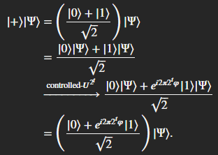
つまり、システム量子ビットの状態は変化せず、の位相が補助量子ビットの状態に「キックバック」されたことになる。
さて、次のことに注意してほしい。

最後の等式では、任意の整数nに対してであるため、位相の「10進数」表現の整数部分は消えている。たとえば、
t=0の場合、位相は
t=1の場合、位相は
t=2の場合、位相は
t=m-1の場合、位相は
最後のt=m-1の場合、位相はとなり、
の場合は1、
の場合は-1となる。最初のケースでは、補助量子ビットq0は|+⟩状態にあり、2番目のケースでは|-⟩状態にある。したがって、Pauli X基底で量子ビットを測定すれば、最初のケースでは0を測定し、2番目のケースでは1を測定するようになり、100%の成功率でこれらのケースを区別できる。測定されたビットは
に等しくなる。
Pauli X基底での測定は、量子ビットを測定する前にアダマールゲートを実行することで行われる。
実装
固有値を持つ固有状態|Ψ⟩=|1⟩を使う。つまり𝜑=1/4=0.01=0.𝜑1𝜑2となる。
𝜑は2ビットで正確に表現できるので、量子回路の実装では2ビットの古典レジスタを使う。
q0が補助量子ビット、q1が|Ψ⟩。
ex1
UゲートとしてSゲートを使って反復位相推定を行う。
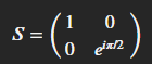
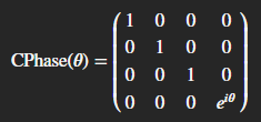
controlled-SゲートはCPhaseGateを使えば良い。
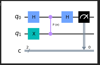
from qiskit import ClassicalRegister, QuantumCircuit, QuantumRegister
import numpy as np


def step_1_circuit(qr: QuantumRegister, cr: ClassicalRegister) -> QuantumCircuit:
    # qr is a quantum register with 2 qubits
    # cr is a classical register with 2 bits

    qc = QuantumCircuit(qr, cr)

    ####### your code goes here #######
    qc.h(0)
    qc.x(1)
    qc.cp(np.pi, 0, 1)
    qc.h(0)
    qc.measure(0,0)

    return qc


qr = QuantumRegister(2, "q")
cr = ClassicalRegister(2, "c")
qc = QuantumCircuit(qr, cr)
qc = step_1_circuit(qr, cr)
qc.draw("mpl")
ex2
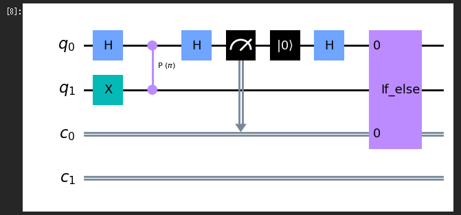
def step_2_circuit(qr: QuantumRegister, cr: ClassicalRegister) -> QuantumCircuit:
    # qr is a quantum register with 2 qubits
    # cr is a classical register with 2 bits

    # begin with the circuit from Step 1
    qc = step_1_circuit(qr, cr)

    ####### your code goes here #######
    qc.reset(qr[0])
    qc.h(qr[0])
    with qc.if_test((cr[0], 0)) as else_:
        # 0を測定したら、正しいので何もしない
        pass
    with else_:
        # 1を測定したら、-pi/2で位相補正する
        qc.rz(-np.pi/2, qr[0])

    return qc


qr = QuantumRegister(2, "q")
cr = ClassicalRegister(2, "c")
qc = QuantumCircuit(qr, cr)
qc = step_2_circuit(qr, cr)
qc.draw("mpl")
さて、この回路をAerSimulatorで実行してみる。
from qiskit_aer import AerSimulator

sim = AerSimulator()
job = sim.run(qc, shots=1000)
result = job.result()
counts = result.get_counts()
counts
# {'01': 1000}
結果は 01 となり、𝜑=1/4=0.01=0.𝜑1𝜑2 を正しく推定できる回路を作ることができた。
ex3
Tゲートの位相を推定するIPEを作れという問題。
これ以降は以前の問題と同じと気づいたので詳細は省略。この回路は何ビット必要か?固有状態は?など、詳しくはIBM Quantum Challenge: Spring 2023 参加記録のLab3のExercise 3を参照。
TゲートのIPE回路は以下になる。
from qiskit import ClassicalRegister, QuantumCircuit, QuantumRegister
import numpy as np


def t_gate_ipe_circuit(qr: QuantumRegister, cr: ClassicalRegister) -> QuantumCircuit:
    # qr is a quantum register with 2 qubits
    # cr is a classical register with 3 bits

    qc = QuantumCircuit(qr, cr)

    ####### your code goes here #######
    """𝜑1のステップ"""
    # 初期化
    qc.h(qr[0])
    qc.x(qr[1])

    # 𝜑1の推定
    qc.cp(np.pi, qr[0], qr[1])
    qc.h(qr[0])
    qc.measure(qr[0], cr[0])

    """𝜑2のステップ"""
    # 初期化
    qc.reset(qr[0])
    qc.h(qr[0])

    # Z軸周りの角度wの回転で位相補正
    with qc.if_test((cr[0], 1)):
        qc.p(-2*np.pi/(2**2), qr[0])

    # 𝜑2の推定
    qc.cp(np.pi/(2**1), qr[0], qr[1])
    qc.h(qr[0])
    qc.measure(qr[0], cr[1])

    """𝜑3のステップ"""
    # 初期化
    qc.reset(qr[0])
    qc.h(qr[0])

    # Z軸周りの角度wの回転で位相補正
    with qc.if_test((cr[0], 1)):
        qc.p(-2*np.pi/(2**3), qr[0])
    with qc.if_test((cr[1], 1)):
        qc.p(-2*np.pi/(2**2), qr[0])

    # 𝜑3の推定
    qc.cp(np.pi/(2**2), qr[0], qr[1])
    qc.h(qr[0])
    qc.measure(qr[0], cr[2])

    return qc


qr = QuantumRegister(2, "q")
cr = ClassicalRegister(3, "c")
qc = QuantumCircuit(qr, cr)
qc = t_gate_ipe_circuit(qr, cr)
qc.draw("mpl")
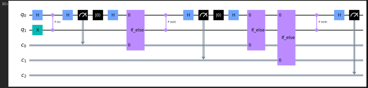
from qiskit_aer import AerSimulator

sim = AerSimulator()
job = sim.run(qc, shots=1000)
result = job.result()
counts = result.get_counts()
counts
# {'001': 1000}
ex4
詳しくはIBM Quantum Challenge: Spring 2023 参加記録のLab3のExercise 4を参照。
ex5
詳しくはIBM Quantum Challenge: Spring 2023 参加記録のLab3のExercise 5を参照。
ex6(ungraded)
ここまでに構築したIPE回路は、特定のゲートと特定の精度ビット数用に設計されたものであった。ここで一般化して、異なるゲートと精度レベルを扱える一般的なIPEルーチンを実装してみよう。
次の関数を完成させて、一般化された IPE ルーチンを実装しよう。以下の入力を受け取る:
qr: 量子レジスタ。最初の量子ビットは補助量子ビット、残りはシステム量子ビットとする。cr: 古典レジスタ。長さは希望する精度のビット数を示す。controlled_unitaries:t=0,...,m-1に対してcontrolled-を実装したゲートのリスト。
state_prep:システム量子ビットの状態を初期化するためのゲート。
from qiskit.circuit import Gate


def iterative_phase_estimation(
    qr: QuantumRegister,
    cr: ClassicalRegister,
    controlled_unitaries: list[Gate],
    state_prep: Gate,
) -> QuantumCircuit:
    qc = QuantumCircuit(qr, cr)

    ####### your code goes here #######
    for i, u_gate in enumerate(controlled_unitaries[::-1]):
        # リセット処理
        if i != 0:
            qc.reset(qr[0])

        qc.h(qr[0])
        if i == 0:
            qc.x(qr[1])
        else:
            # Z軸周りの角度wの回転で位相補正
            for j in range(0, i):
                with qc.if_test((cr[j], 1)):
                    qc.p(-np.pi /(2**(i-j)), qr[0])

        qc.append(u_gate, [qr[0], qr[1]])

        # X基底でq0を測定
        qc.h(qr[0])
        qc.measure(qr[0], cr[i])

    return qc
この関数を使用してS ゲートのIPE回路を生成する。
from qiskit.circuit.library import CPhaseGate, XGate

qr = QuantumRegister(2, "q")
cr = ClassicalRegister(2, "c")

s_angle = np.pi / 2
controlled_unitaries = [CPhaseGate(s_angle * 2**k) for k in range(2)]
qc = iterative_phase_estimation(qr, cr, controlled_unitaries, XGate())
qc.draw()
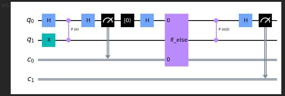
回路を実行する。結果は01になるはずである。
sim = AerSimulator()
job = sim.run(qc, shots=1000)
result = job.result()
counts = result.get_counts()
counts
# {'01': 1000}
合ってる。
Tゲートでも検証してみる。
qr = QuantumRegister(2, "q")
cr = ClassicalRegister(3, "c")

t_angle = np.pi / 4
controlled_unitaries = [CPhaseGate(t_angle * 2**k) for k in range(3)]
qc = iterative_phase_estimation(qr, cr, controlled_unitaries, XGate())
qc.draw()
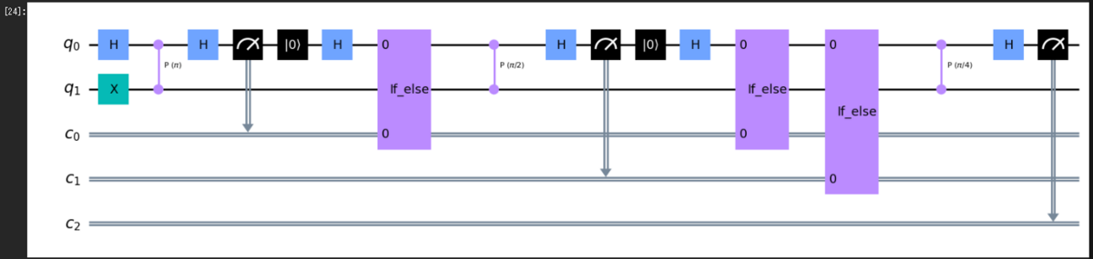
回路を実行する。結果は001になるはずである。
sim = AerSimulator()
job = sim.run(qc, shots=1000)
result = job.result()
counts = result.get_counts()
counts
# {'001': 1000}
合ってる。
Qiskit Global Summer School 2023 Lab3 参加記録
各Labの記録
- 参加結果の記事:Qiskit Global Summer School 2023 参加記録
- Lab1:記事なし。かなり基礎的な内容だった気がするので
- Lab2:Qiskit Global Summer School 2023 Lab2 参加記録
- Lab3:Qiskit Global Summer School 2023 Lab3 参加記録
- Lab4:Qiskit Global Summer School 2023 Lab4 参加記録
- Lab5:Qiskit Global Summer School 2023 Lab5 参加記録
まえがき
Qiskit Global Summer School 2023 Lab3の記録です。
Lab 3 : Diving Into Quantum Algorithms
ex1
5量子ビット(位相推定用のビット数4 + 補助量子ビット数1個)のQPE回路を作る問題。以下の回路を作れば良い。
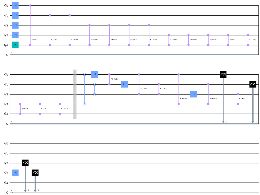
QFTと逆QFTのサンプルコードは与えられているので、それらを使って作ることができる。
#QFT Circuit
def qft(n):
    """Creates an n-qubit QFT circuit"""
    circuit = QuantumCircuit(n)
    def swap_registers(circuit, n):
        for qubit in range(n//2):
            circuit.swap(qubit, n-qubit-1)
        return circuit
    def qft_rotations(circuit, n):
        """Performs qft on the first n qubits in circuit (without swaps)"""
        if n == 0:
            return circuit
        n -= 1
        circuit.h(n)
        for qubit in range(n):
            circuit.cp(np.pi/2**(n-qubit), qubit, n)
        qft_rotations(circuit, n)

    qft_rotations(circuit, n)
    swap_registers(circuit, n)
    return circuit

#Inverse Quantum Fourier Transform
def qft_dagger(qc, n):
    """n-qubit QFTdagger the first n qubits in circ"""
    # Don't forget the Swaps!
    for qubit in range(n//2):
        qc.swap(qubit, n-qubit-1)
    for j in range(n):
        for m in range(j):
            qc.cp(-np.pi/float(2**(j-m)), m, j)
        qc.h(j)
    return qc
phase_register_size = 4
qpe4 = QuantumCircuit(phase_register_size+1, phase_register_size)

### Insert your code here
# Preparation
for i in range(4):
    qpe4.h(i)
qpe4.x(4)

# Apply CP Gate
angle = np.pi*2/3 # λ
for i in range(4):
    for _ in range(2**i):
        qpe4.cp(angle, i, 4)
qpe4.barrier()

# Apply QFT^dagger
qpe4 = qft_dagger(qpe4, 4)

# Measure
for i in range(0, 4):
    qpe4.measure(i, i)

qpe4.draw()
シミュレータ実行すると以下が得られた。
## Run this cell to simulate 'qpe4' and to plot the histogram of the result
sim = Aer.get_backend('aer_simulator')
shots = 2000
count_qpe4 = execute(qpe4, sim, shots=shots).result().get_counts()
plot_histogram(count_qpe4, figsize=(9,5))
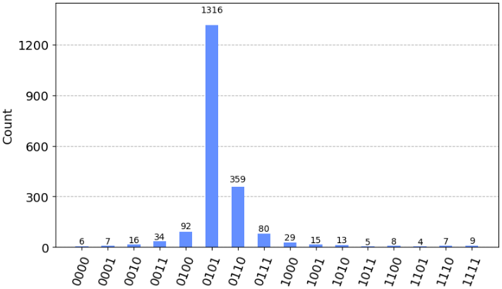
結果は 0101 が最も大きい確率となった。
位相推定の結果 は、
- N: 最も確率が高かった値(10進数)
- n: 位相推定用のビット数
とすると、 で求めることができる。詳しくはSampler primitive を使用した量子位相推定に書いてある。
2進数の 0101 は10進数で 5 なので位相推定の結果は、
estimated_phase = 5/(2**phase_register_size)
print("estimated_phase: ", estimated_phase)
print("誤差: ", abs(estimated_phase - 1/3))
# estimated_phase:  0.3125
# 誤差:  0.020833333333333315
となる。たしかに真値θ = 1/3 (=0.3333...) に近い値を推定できたということになる。
余談だが、今の状態で更に精度を上げるにはSampler primitive を使用した量子位相推定#ステップ-3:-結果の分析に書いてあるように、2番目に確率が大きい値との加重平均を取ればいい(最も確率が大きい値の近傍になっていることが望ましい)。
今回の場合で言えば2番目に確率が大きいのは 0110 (10進数で6)であり、最も確率が高い5の近傍であるので適している。加重平均をとった結果は以下になる。
# 2番目に確率が大きい値との加重平均をとると更に良さそう
estimated_phase1 = 5/(2**phase_register_size)
estimated_phase2 = 6/(2**phase_register_size)
estimated_phase = (estimated_phase1+estimated_phase2)/2
print("estimated_phase: ", estimated_phase)
print("誤差: ", abs(estimated_phase - 1/3))
# estimated_phase:  0.34375
# 誤差:  0.010416666666666685
簡単に真値θ = 1/3 (=0.3333...)との誤差を小さくすることができた。
ex2
- 位相推定の結果は何?
- この回路は最大で2の何乗までの精度を計算できるか?
の2つを答える問題。2番目の答えの意味を汲むのが少しむずかしかった。

今回位相推定用のビット数tは4なので、 までの精度を計算できる。
#Grab the highest probability measurement
max_binary_counts = 0
max_binary_val = ''
for key, item in count_qpe4.items():
    if item > max_binary_counts:
        max_binary_counts = item
        max_binary_val = key

## Your function to convert a binary string to decimal goes here
# calculate the estimated phase
dec = 0
for i, c in enumerate(max_binary_val[::-1]):
    dec += (2**i) * int(c)
estimated_phase = dec/(2**phase_register_size)
print("estimated_phase: ", estimated_phase)

# highest power of 2 (i.e. smallest decimal) this circuit can estimate
phase_accuracy_window = 1/(2**4)
print("phase_accuracy_window: ", phase_accuracy_window)
ex3

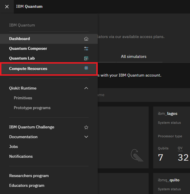
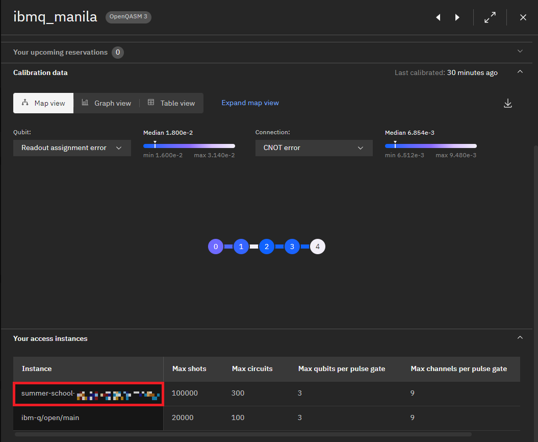
実機情報を得るために provider_get_backend() する必要があるのだが、引数に渡す hub, group, project がなんなのか分からなくて困った。Discordに書いてあった。
For the hub, group, and project, From main page menu of IBM Quantum Experience portal -> Computer Resources - > Your Resources ( Select Table view from right)- > click on ibmq_manila -> go to the section Your Access Instance -> Details will be in a string of format summer-school-x/group-x/xxxxxxxxxx
Qiskitはデフォルトで確率的スワップマッパーを使用して必要なSWAPゲートを配置するため、同じランタイム設定であってもトランスパイルされた回路結果にばらつきが生じる。回路深度の短いトランスパイル回路の方が結果の誤差は小さくなるので、qpe4を複数回トランスパイルして回路深度が最小のものを選ぶ必要がある。
transpile方法は qiskit.compiler.transpile に書いてある。
from qiskit_ibm_provider import IBMProvider
from qiskit.compiler import transpile

# summer-school-x/group-x/xxxxxxxxxx
provider = IBMProvider()
hub = "summer-school-x"
group = "group-x"
project = "xxxxxxxxxx"
backend_name = "ibmq_manila"

backend = provider.get_backend(backend_name, instance=f"{hub}/{group}/{project}")

# your code goes here
# 適当に100回トランスパイルして、最も深い回路と最も浅い回路をそれぞれ得る
max_depth = 0
min_depth = 999
min_depth_qpe = None
max_depth_qpe = None
for _ in range(100):
    transpiled_qc = transpile(circuits=qpe4, backend=backend, optimization_level=3)
    if transpiled_qc.depth() > max_depth:
        max_depth = transpiled_qc.depth()
        max_depth_qpe = transpiled_qc
    if transpiled_qc.depth() < min_depth:
        min_depth = transpiled_qc.depth()
        min_depth_qpe = transpiled_qc
print("min_depth_qpe.depth(): ", min_depth_qpe.depth())
print("max_depth_qpe.depth(): ", max_depth_qpe.depth())
# min_depth_qpe.depth():  75
# max_depth_qpe.depth():  78
最も浅い回路を実行してみる。
shots = 2000

#OPTIONAL: Run the minimum depth qpe circuit
job_min_qpe4 = backend.run(min_depth_qpe, sim, shots=shots)
print(job_min_qpe4.job_id())

#Gather the count data
count_min_qpe4 = job_min_qpe4.result().get_counts()
plot_histogram(count_min_qpe4, figsize=(9,5))
cj6rcddtks61ugsn95hg
Traceback (most recent call last):
  Cell In[86], line 8
    count_min_qpe4 = job_min_qpe4.result().get_counts()
  File /opt/conda/lib/python3.10/site-packages/qiskit_ibm_provider/job/ibm_circuit_job.py:250 in result
    raise IBMJobFailureError(f"Job failed: " f"{error_message}")
IBMJobFailureError: 'Job failed: Internal Error while executing OpenQASM 3 circuit.'

Use %tb to get the full traceback.
なんかエラーが出て実行できなかったので、代わりにFakeManilaV2を使ったシミュレータ実行をした。
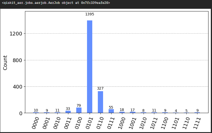
最も浅い回路の実行結果は以下になった。
# なんか実機のバックエンド実行でエラーが出たので、しょうがないのでシミュレータを使って実行する
from qiskit.providers.fake_provider import FakeManilaV2
backend_fakemanilav2 = FakeManilaV2()

shots = 2000

#OPTIONAL: Run the minimum depth qpe circuit
job_min_qpe4 = sim.run(min_depth_qpe, backend=backend_fakemanilav2, shots=shots)
print(job_min_qpe4.job_id())

#Gather the count data
print(job_min_qpe4)
count_min_qpe4 = job_min_qpe4.result().get_counts()
plot_histogram(count_min_qpe4, figsize=(9,5))
最も深い回路の実行結果は以下になった。
# こちらもシミュレータを使って実行する
job_max_qpe4 = sim.run(max_depth_qpe, backend=backend_fakemanilav2, shots=shots)
print(job_max_qpe4.job_id())

#Gather the count data
count_max_qpe4 = job_max_qpe4.result().get_counts()
plot_histogram(count_max_qpe4, figsize=(9,5))
min_depth_qpeの方が0101の確率が高いので、(誤差の範疇の気もするが)たしかに精度が高いと言える。
ex4

「真値θ=1/7 としたときの位相推定をするとき、誤差が2^-6以下になるのに必要な最小の位相推定用のビット数は?」という問題。
位相推定用のビット数register_sizeを指定してQPE回路を作る関数は以下のようにする。
Pゲートのλの値はどうするか?

ちなみに「Pゲートのλの値を決めるためには推定すべきθの値を知ってないといけないのはどういうことやねん。意味あんのか?」という疑問はもっともである。この疑問は因数分解ソルバーであるショアのアルゴリズムが少し解消してくれる。
さらにちなみに、Qiskit Textbook の量子位相推定ではPゲートの代わりにTゲートを使っているが、考え方は同じである。
def qpe_circuit(register_size):
    # Your code goes here
    qpe = QuantumCircuit(register_size+1, register_size)

    # Preparation
    for i in range(register_size):
        qpe.h(i)
    qpe.x(register_size)

    # Apply CP Gate
    angle = np.pi*2/7 # λ
    for i in range(register_size):
        for _ in range(2**i):
            qpe.cp(angle, i, register_size)
    qpe.barrier()

    # Apply QFT^dagger
    qpe = qft_dagger(qpe, register_size)

    # Measure
    for i in range(0, register_size):
        qpe.measure(i, i)

    return qpe
位相推定用のビット数 reg_size=6 としたときの結果は以下のようになった。
## Run this cell to simulate 'qpe4' and to plot the histogram of the result
reg_size = 6# Vary the register sizes

qpe_check = qpe_circuit(reg_size)
sim =  Aer.get_backend('aer_simulator')
shots = 10000
count_qpe4 = execute(qpe_check, sim, shots=shots).result().get_counts()
plot_histogram(count_qpe4, figsize=(19,5))
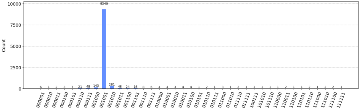
真値との誤差を計算する関数を以下のように作った。
# 真値との誤差を計算する関数
def calc_error(count_qpe):
    #Grab the highest probability measurement
    max_binary_counts = 0
    max_binary_val = ''
    for key, item in count_qpe.items():
        if item > max_binary_counts:
            max_binary_counts = item
            max_binary_val = key

    ## Your function to convert a binary string to decimal goes here
    # calculate the estimated phase
    dec = 0
    for i, c in enumerate(max_binary_val[::-1]):
        dec += (2**i) * int(c)
    estimated_phase = dec/(2**reg_size)
    print("estimated_phase: ", estimated_phase)

    # 真値
    true_phase = 1/7
    print("true phase: ", true_phase)

    # 誤差
    error = abs(estimated_phase-true_phase)
    print("誤差: ", error)

    return error
さて、誤差が2^-6以下となるような最小のビット数を求めたい。1から順に回して調べればよい。
# 誤差が2^-6以下になるために必要な最小のビット数は?
required_register_size = 1
for n in range(1, 100):
    print("===register_size:{}===".format(n))
    reg_size = n# Vary the register sizes

    qpe_check = qpe_circuit(reg_size)
    sim =  Aer.get_backend('aer_simulator')
    shots = 10000
    count_qpe = execute(qpe_check, sim, shots=shots).result().get_counts()

    error = calc_error(count_qpe)

    # 誤差が2^-6以下になったら終了
    if error <= 2**(-6):
        required_register_size = n
        break
print(required_register_size)
===register_size:1===
estimated_phase:  0.0
true phase:  0.14285714285714285
誤差:  0.14285714285714285
===register_size:2===
estimated_phase:  0.25
true phase:  0.14285714285714285
誤差:  0.10714285714285715
===register_size:3===
estimated_phase:  0.125
true phase:  0.14285714285714285
誤差:  0.01785714285714285
===register_size:4===
estimated_phase:  0.125
true phase:  0.14285714285714285
誤差:  0.01785714285714285
===register_size:5===
estimated_phase:  0.15625
true phase:  0.14285714285714285
誤差:  0.01339285714285715
5
ということで5が正解。
ex5
テーマはショアのアルゴリズムの実装に移る。
ショアのアルゴリズムのQiskitの記事が消えてて(検索してもいいのが出てこなかった)困ったのだが、 素因数分解アルゴリズムを学習する — 量子コンピューティング・ワークブック の記事がわかりやすかったのでそれを参考にした。
さて、Uゲートとして 「7mod15ゲート」を作ったので、それが正しく動作するかチェックしようという問題。
### your code goes here

# |1>で確認する
qcirc = QuantumCircuit(m)
qcirc.x(0)
qcirc.append(U, [i for i in range(m)])
qcirc.measure_all()
qcirc.draw()

# |2>で確認する
qcirc2 = QuantumCircuit(m)
qcirc2.x(1)
qcirc2.append(U, [i for i in range(m)])
qcirc2.measure_all()
qcirc2.draw()

# |5>で確認する
qcirc5 = QuantumCircuit(m)
qcirc5.x(0)
qcirc5.x(2)
qcirc5.append(U, [i for i in range(m)])
qcirc5.measure_all()
qcirc5.draw()

回答コードは以下。
## Run this cell to simulate 'qpe4' and to plot the histogram of the result
sim = Aer.get_backend('aer_simulator')
shots = 20000

input_1 = execute(qcirc, sim, shots=shots).result().get_counts()  # save the count data for input 1

input_2 = execute(qcirc2, sim, shots=shots).result().get_counts()# save the count data for input 2
input_5 = execute(qcirc5, sim, shots=shots).result().get_counts()# save the count data for input 5
input_1をヒストグラムで表示すると、以下になった。
plot_histogram(input_1, figsize=(10,5))
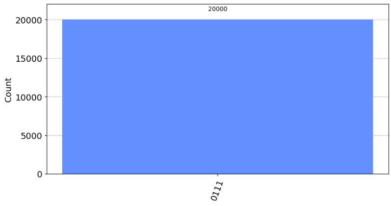
1*7 mod 15 ≡ 7(0111) なので、正しい結果が得られている。
他2つの結果も載せておく。どれも正しい結果が得られているので、正しく実装できたようだ。
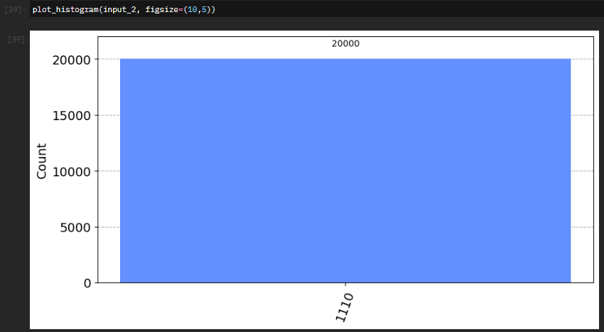
2*7 mod 15 ≡ 14(1110)

5*7 mod 15 ≡ 5(0101)
ex6
7mod15ゲートは4回適用するとIゲートと同じということを確認する問題。
たしかに、7 * 7 * 7 * 7 ≡ 1 (mod 15) なので、その通りである。
unitary_circ = QuantumCircuit(m)

# Your code goes here
for i in range(4):
    unitary_circ.append(U, [i for i in range(m)])

unitary_circ.draw()
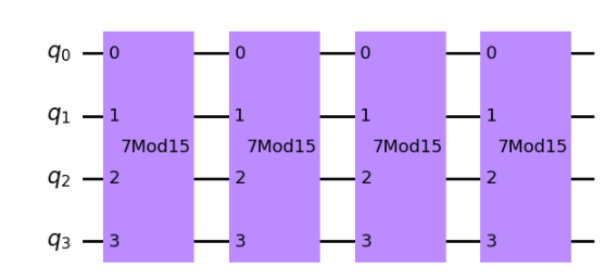
回路を unitary_simulator で実行して、結果をユニタリ行列化したものを見てみよう。
sim = Aer.get_backend('unitary_simulator')
unitary = execute(unitary_circ, sim).result().get_unitary()
print(unitary)
Operator([[1.+0.j, 0.+0.j, 0.+0.j, 0.+0.j, 0.+0.j, 0.+0.j, 0.+0.j, 0.+0.j,
           0.+0.j, 0.+0.j, 0.+0.j, 0.+0.j, 0.+0.j, 0.+0.j, 0.+0.j, 0.+0.j],
          [0.+0.j, 1.+0.j, 0.+0.j, 0.+0.j, 0.+0.j, 0.+0.j, 0.+0.j, 0.+0.j,
           0.+0.j, 0.+0.j, 0.+0.j, 0.+0.j, 0.+0.j, 0.+0.j, 0.+0.j, 0.+0.j],
          [0.+0.j, 0.+0.j, 1.+0.j, 0.+0.j, 0.+0.j, 0.+0.j, 0.+0.j, 0.+0.j,
           0.+0.j, 0.+0.j, 0.+0.j, 0.+0.j, 0.+0.j, 0.+0.j, 0.+0.j, 0.+0.j],
          [0.+0.j, 0.+0.j, 0.+0.j, 1.+0.j, 0.+0.j, 0.+0.j, 0.+0.j, 0.+0.j,
           0.+0.j, 0.+0.j, 0.+0.j, 0.+0.j, 0.+0.j, 0.+0.j, 0.+0.j, 0.+0.j],
          [0.+0.j, 0.+0.j, 0.+0.j, 0.+0.j, 1.+0.j, 0.+0.j, 0.+0.j, 0.+0.j,
           0.+0.j, 0.+0.j, 0.+0.j, 0.+0.j, 0.+0.j, 0.+0.j, 0.+0.j, 0.+0.j],
          [0.+0.j, 0.+0.j, 0.+0.j, 0.+0.j, 0.+0.j, 1.+0.j, 0.+0.j, 0.+0.j,
           0.+0.j, 0.+0.j, 0.+0.j, 0.+0.j, 0.+0.j, 0.+0.j, 0.+0.j, 0.+0.j],
          [0.+0.j, 0.+0.j, 0.+0.j, 0.+0.j, 0.+0.j, 0.+0.j, 1.+0.j, 0.+0.j,
           0.+0.j, 0.+0.j, 0.+0.j, 0.+0.j, 0.+0.j, 0.+0.j, 0.+0.j, 0.+0.j],
          [0.+0.j, 0.+0.j, 0.+0.j, 0.+0.j, 0.+0.j, 0.+0.j, 0.+0.j, 1.+0.j,
           0.+0.j, 0.+0.j, 0.+0.j, 0.+0.j, 0.+0.j, 0.+0.j, 0.+0.j, 0.+0.j],
          [0.+0.j, 0.+0.j, 0.+0.j, 0.+0.j, 0.+0.j, 0.+0.j, 0.+0.j, 0.+0.j,
           1.+0.j, 0.+0.j, 0.+0.j, 0.+0.j, 0.+0.j, 0.+0.j, 0.+0.j, 0.+0.j],
          [0.+0.j, 0.+0.j, 0.+0.j, 0.+0.j, 0.+0.j, 0.+0.j, 0.+0.j, 0.+0.j,
           0.+0.j, 1.+0.j, 0.+0.j, 0.+0.j, 0.+0.j, 0.+0.j, 0.+0.j, 0.+0.j],
          [0.+0.j, 0.+0.j, 0.+0.j, 0.+0.j, 0.+0.j, 0.+0.j, 0.+0.j, 0.+0.j,
           0.+0.j, 0.+0.j, 1.+0.j, 0.+0.j, 0.+0.j, 0.+0.j, 0.+0.j, 0.+0.j],
          [0.+0.j, 0.+0.j, 0.+0.j, 0.+0.j, 0.+0.j, 0.+0.j, 0.+0.j, 0.+0.j,
           0.+0.j, 0.+0.j, 0.+0.j, 1.+0.j, 0.+0.j, 0.+0.j, 0.+0.j, 0.+0.j],
          [0.+0.j, 0.+0.j, 0.+0.j, 0.+0.j, 0.+0.j, 0.+0.j, 0.+0.j, 0.+0.j,
           0.+0.j, 0.+0.j, 0.+0.j, 0.+0.j, 1.+0.j, 0.+0.j, 0.+0.j, 0.+0.j],
          [0.+0.j, 0.+0.j, 0.+0.j, 0.+0.j, 0.+0.j, 0.+0.j, 0.+0.j, 0.+0.j,
           0.+0.j, 0.+0.j, 0.+0.j, 0.+0.j, 0.+0.j, 1.+0.j, 0.+0.j, 0.+0.j],
          [0.+0.j, 0.+0.j, 0.+0.j, 0.+0.j, 0.+0.j, 0.+0.j, 0.+0.j, 0.+0.j,
           0.+0.j, 0.+0.j, 0.+0.j, 0.+0.j, 0.+0.j, 0.+0.j, 1.+0.j, 0.+0.j],
          [0.+0.j, 0.+0.j, 0.+0.j, 0.+0.j, 0.+0.j, 0.+0.j, 0.+0.j, 0.+0.j,
           0.+0.j, 0.+0.j, 0.+0.j, 0.+0.j, 0.+0.j, 0.+0.j, 0.+0.j, 1.+0.j]],
         input_dims=(2, 2, 2, 2), output_dims=(2, 2, 2, 2))
少し分かりづらいが、単位行列(Iゲートと同値)になっていることがわかる。
ex7
7mod15ゲートをコントロールUゲート化して、QPEをしてみようという問題。
- 位相推定用のビット数は8
- 補助量子ビット数は4
- 固有状態は|1⟩を与える
7mod15ゲートをコントロールUゲート化する関数は以下の関数として与えられている。
#This function will return a ControlledGate object which repeats the action
# of U, 2^k times
def cU_multi(k):
    sys_register_size = 4
    circ = QuantumCircuit(sys_register_size)
    for _ in range(2**k):
        circ.append(U, range(sys_register_size))

    U_multi = circ.to_gate()
    U_multi.name = '7Mod15_[2^{}]'.format(k)

    cU_multi = U_multi.control()
    return cU_multi
回路のコードは以下。
# your code goes here

phase_register_size = 8
sys_register_size = 4
shor_register_size = phase_register_size + sys_register_size


shor_qpe = QuantumCircuit(shor_register_size, phase_register_size) #Create the QuantumCircuit needed to run with 8 phase register qubits

# Step1: Preparation
for i in range(phase_register_size):
    shor_qpe.h(i)
shor_qpe.x(phase_register_size)

# Step2: Apply cU
for i in range(phase_register_size):
    cu = cU_multi(i)
    shor_qpe.append(cu, [i, *[phase_register_size+j for j in range(sys_register_size)]])

# Spte3: Apply inversed-QFT
shor_qpe = qft_dagger(shor_qpe, phase_register_size)

# Step4: Measure phase_register
for i in range(phase_register_size):
    shor_qpe.measure(i, i)

shor_qpe.draw()
aer_simulator で実行して結果を得る。
## Run this cell to simulate 'shor_qpe' and to plot the histogram of the results
sim = Aer.get_backend('aer_simulator')
shots = 20000
shor_qpe_counts = execute(shor_qpe, sim, shots=shots).result().get_counts()
plot_histogram(shor_qpe_counts, figsize=(19,5))
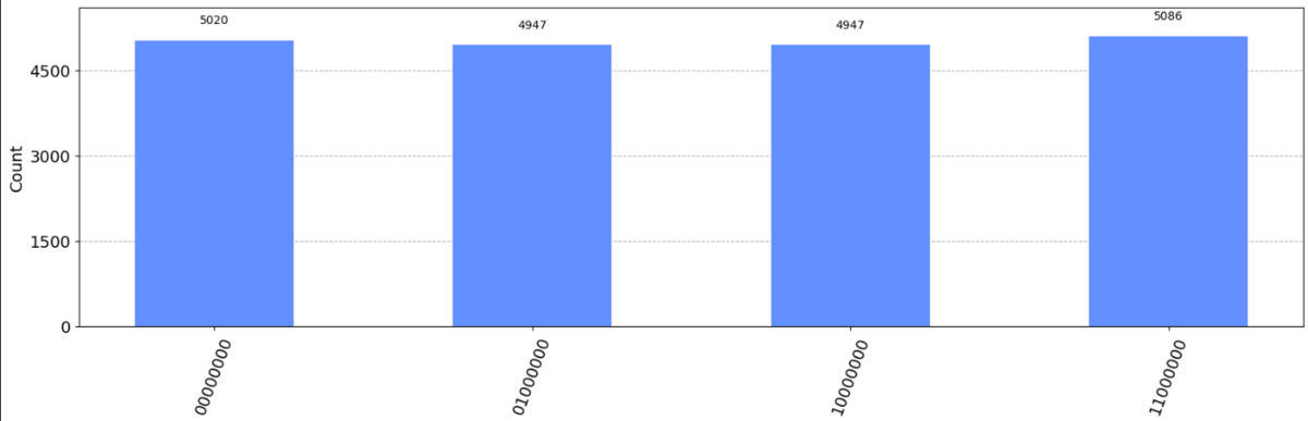
00000000, 01000000, 10000000, 11000000 それぞれの確率がほぼ等確率で得られたので、位相推定の結果は、
# 位相推定の結果
n = 8 # 位相推定用のビット数

estimated_thetas = [] # 推定された位相のリスト
for key, val in shor_qpe_counts.items():
    dec = 0 # 10進数の値
    for i, c in enumerate(key[::-1]):
        dec += (2**i)*int(c)
    estimated_theta = dec/(2**n)
    estimated_thetas.append(estimated_theta)

estimated_thetas.sort()
print(estimated_thetas)
[0.0, 0.25, 0.5, 0.75]
0.0, 0.25, 0.5, 0.75 のどれかという結果が得られた。
ex8
PythonのFractionライブラリを使って、位相推定した結果をs/rという分数で表現せよという問題。今回mod15なのでrは15未満。
from fractions import Fraction
shor_qpe_fractions = []# create a list of Fraction objects for each measurement outcome
for estimated_theta in estimated_thetas:
    shor_qpe_fractions.append(Fraction(estimated_theta).limit_denominator(15))
[Fraction(0, 1), Fraction(1, 4), Fraction(1, 2), Fraction(3, 4)]
ex9
いよいよショアのアルゴリズム全体を実装せよという問題。今まで使った関数やQPEを使えば実装できる。
ショアのアルゴリズムの回路や全体像は素因数分解アルゴリズムを学習する — 量子コンピューティング・ワークブックがわかりやすかったので、それを参考にして実装した。
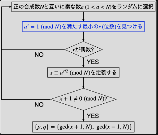
今回は7mod15ゲートのみを使うので、a=7で固定とする。
グレーダーにバグがあるっぽく、以下を実行してアップデートしたあと、カーネルを再起動する必要がある。
!pip install git+https://github.com/qiskit-community/Quantum-Challenge-Grader.git@main
"""ショアのQPE回路を作成する"""
def shor_qpe_circuit():
    phase_register_size = 8
    sys_register_size = 4
    shor_register_size = phase_register_size + sys_register_size

    shor_qpe = QuantumCircuit(shor_register_size, phase_register_size) #Create the QuantumCircuit needed to run with 8 phase register qubits

    # Step1: Preparation
    for i in range(phase_register_size):
        shor_qpe.h(i)
    shor_qpe.x(phase_register_size)

    # Step2: Apply cU
    for i in range(phase_register_size):
        cu = cU_multi(i)
        shor_qpe.append(cu, [i, *[phase_register_size+j for j in range(sys_register_size)]])

    # Spte3: Apply inversed-QFT
    shor_qpe = qft_dagger(shor_qpe, phase_register_size)

    # Step4: Measure phase_register
    for i in range(phase_register_size):
        shor_qpe.measure(i, i)

    return shor_qpe
"""位相推定の結果を返す"""
def calc_estimated_phases(shor_qpe_counts):
    n = 8 # 位相推定用のビット数

    estimated_thetas = [] # 推定した位相のリスト
    for key, val in shor_qpe_counts.items():
        dec = 0 # 10進数の値
        for i, c in enumerate(key[::-1]):
            dec += (2**i)*int(c)
        estimated_theta = dec/(2**n)
        estimated_thetas.append(estimated_theta)

    # estimated_thetas.sort()
    return estimated_thetas
def shor_qpe(k):

    a = 7
    N = 15
    #Step 1. Begin a while loop until a nontrivial guess is found
    ### Your code goes here ###
    trivial_r = set() # だめだったrを保存しておく
    cnt = 0 # ループ回数
    while 1:
        cnt += 1
        if cnt == 20:
            # 無限ループを回避したい(20回やって駄目なら失敗とする)
            print("Not Found!!!!")
            break

        #Step 2a. Construct a QPE circuit with m phase count qubits
        #  to guess the phase phi = s/r using the function cU_multi()
        ### Your code goes here ###
        qpe_qc = shor_qpe_circuit()

        #Step 2b. Run the QPE circuit with a single shot, record the results
        # and convert the estimated phase bitstring to decimal
        ### Your code goes here ###
        sim = Aer.get_backend('aer_simulator')
        shots = 1 # シングルショットなので結果は1個だけなことに注意
        shor_qpe_counts = execute(qpe_qc, sim, shots=shots).result().get_counts()
        estimated_phases = calc_estimated_phases(shor_qpe_counts)

        #Step 3. Use the Fraction object to find the guess for r
        ### Your code goes here ###
        shor_qpe_fraction = Fraction(estimated_phases[0]).limit_denominator(15)
        r = shor_qpe_fraction.denominator
        if r in trivial_r:
            continue
        trivial_r.add(r)

        #Step 4. Now that r has been found, use the builtin greatest common deonominator
        # function to determine the guesses for a factor of N
        guesses = [gcd(a**(r//2)-1, N), gcd(a**(r//2)+1, N)]

        #Step 5. For each guess in guesses, check if at least one is a non-trivial factor
        # i.e.  (guess != 1 or N) and (N % guess == 0)
        ### Your code goes here ###
        is_ok = True
        for guess in guesses:
            if guess==1 or guess==N or N%guess!= 0:
                is_ok = False
        if guesses[0]*guesses[1] != N:
            is_ok = False
        if is_ok:
            break

    #Step 6. If a nontrivial factor is found return the list 'guesses', otherwise
    # continue the while loop
    ### Your code goes here ###
    print("ループ回数:", cnt)
    return guesses
実行結果。
m = 4
guesses = shor_qpe(m)
print(guesses)
ループ回数: 2
[3, 5]
(結構グレーダーゆるゆるで、N=15の素因数分解の答えとして[15, 1]を返すような関数でもパスした)
Qiskit Global Summer School 2023 Lab2 参加記録
各Labの記録
- 参加結果の記事:Qiskit Global Summer School 2023 参加記録
- Lab1:記事なし。かなり基礎的な内容だった気がするので
- Lab2:Qiskit Global Summer School 2023 Lab2 参加記録
- Lab3:Qiskit Global Summer School 2023 Lab3 参加記録
- Lab4:Qiskit Global Summer School 2023 Lab4 参加記録
- Lab5:Qiskit Global Summer School 2023 Lab5 参加記録
まえがき
Qiskit Global Summer School 2023 Lab2の記録です。
Lab2
ex1
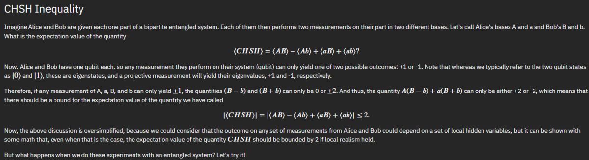
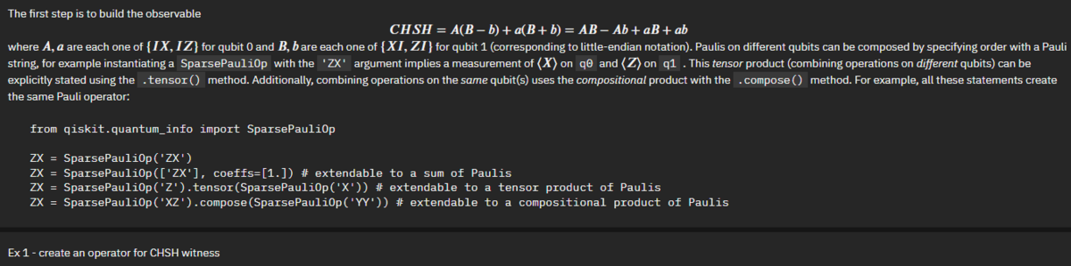
IX = SparsePauliOp("IX")
XI = SparsePauliOp("XI")
IZ = SparsePauliOp("IZ")
ZI = SparsePauliOp("ZI")

# 「Aはq0にIX演算をする」、「Bはq1にXI演算をする」とすると、ABはXX演算になる。
AB = SparsePauliOp("XX")
Ab = SparsePauliOp("ZX")
aB = SparsePauliOp("XZ")
ab = SparsePauliOp("ZZ")
提出コードは以下。
obsv = AB - Ab + aB + ab# create operator for chsh witness
obsv
# SparsePauliOp(['XX', 'ZX', 'XZ', 'ZZ'],
#               coeffs=[ 1.+0.j, -1.+0.j,  1.+0.j,  1.+0.j])
ex2

|<CHSH>| > 2 となるθを4つ探せという問題。マンデルブロ集合かな?
Demonstrate the violation of the CHSH inequality with the Estimator primitiveを参考にしつつ答えを探した。
まず[-2π, 2π]の区間で角度を100分割したものを作る。
angles = []
diff = np.pi*4/100
for i in range(0, 100):
    angles.append([-2*np.pi+diff*i])
すると以下のようなグラフが得られた。
estimator = Estimator()
job = estimator.run([qc]*len(angles), observables=[obsv]*len(angles), parameter_values=angles)
exps = job.result().values

plt.plot(angles, exps, marker='x', ls='-', color='green')
plt.plot(angles, [2]*len(angles), ls='--', color='red', label='Classical Bound')
plt.plot(angles, [-2]*len(angles), ls='--', color='red')
plt.xlabel('angle (rad)')
plt.ylabel('CHSH Witness')
plt.legend(loc=4)
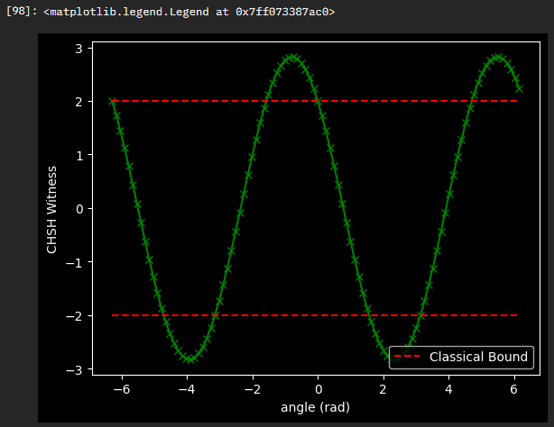
このグラフを眺めて答えを提出した。例えば i=13, 14, 15, 16 のときにCHSHの破れが起きているので、以下のコードを提出すればよい。
# i=[13, 16] が破れているので、以下を答えとして提出する
angles = []
diff = np.pi*4/100
for i in range(13, 17):
    angles.append([-2*np.pi+diff*i])
ex3

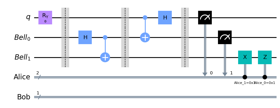
このエクササイズでやることは、
ということをすればいい。
条件付きゲート: c_if メソッド を使って実装できる。
graded_qc = tele_qc.copy()

##############################
# add gates to graded_qc here

graded_qc.x(bell[1]).c_if(alice[1], 1)
graded_qc.z(bell[1]).c_if(alice[0], 1)

##############################

graded_qc.draw('mpl')
ex4

Statevector は動的回路では使えないので、 Samplerを使って量子テレポーテーション回路を実行する。
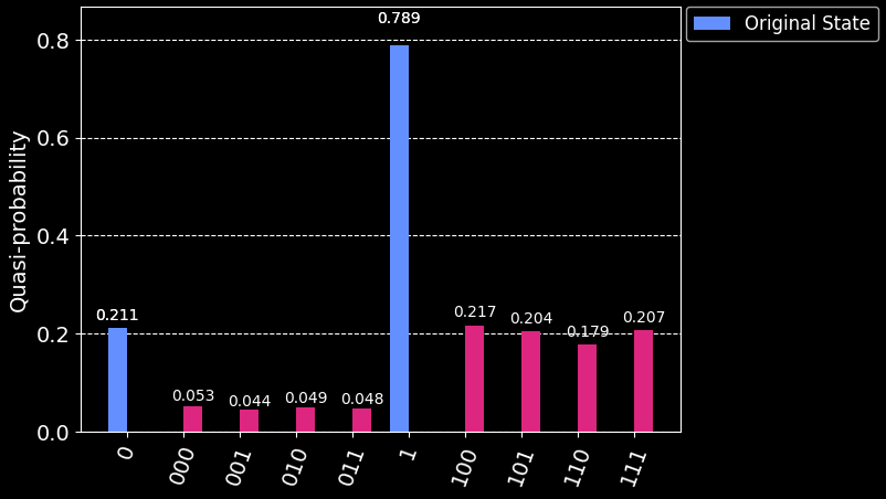
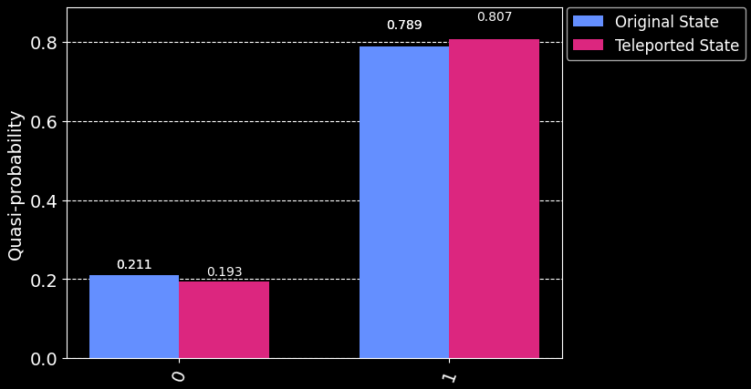
θ=5π/7として実行すると、1が80%、0が20%の確率で測定される。
from qiskit_aer.primitives import Sampler

angle = 5*np.pi/7

sampler = Sampler()
qc.measure_all()
job_static = sampler.run(qc.bind_parameters({theta: angle}))
job_dynamic = sampler.run(graded_qc.bind_parameters({theta: angle}))

print(f"Original Dists: {job_static.result().quasi_dists[0].binary_probabilities()}")
print(f"Teleported Dists: {job_dynamic.result().quasi_dists[0].binary_probabilities()}")
# Original Dists: {'0': 0.2109375, '1': 0.7890625}
# Teleported Dists: {'001': 0.0439453125, '000': 0.052734375, '010': 0.048828125, '110': 0.1787109375, '101': 0.2041015625, '100': 0.216796875, '011': 0.0478515625, '111': 0.20703125}
今回のエクササイズは、「得られた Teleported Dists の結果を、Original Dists と同じ確率分布になるように周辺化せよ」という問題。
ここで周辺化(Marginalize)とは、6. 確率・統計の基礎 — ディープラーニング入門によると、
同時確率が与えられたとき、着目していない方の確率変数がとり得る全ての値について同時確率を計算しその和をとることを周辺化 (marginalization) と呼び、結果として得られる確率を周辺確率 (marginal probability) と呼びます
とある。
今回の場合では、Bobの量子ビット(2番目のビット)だけに着目したいのであって、それ以外の量子ビットは興味ない。ので、
- 100, 101, 110, 111 を1に周辺化する
- 000, 001, 010, 011 を0に周辺化する
とすればよい。
得られた周辺確率分布は Original State の確率分布とほぼ等しくなるはずである。
まず、周辺化前の分布を比較すると以下になった。
legend = ['Original State', 'Teleported State']
plot_histogram([job_static.result().quasi_dists[0].binary_probabilities(), job_dynamic.result().quasi_dists[0].binary_probabilities()], legend=legend)
この確率分布を周辺化する。周辺化には qiskit.result.marginal_counts ライブラリを使えば良い。
from qiskit.result import marginal_counts

tele_counts = marginal_counts(job_dynamic.result().quasi_dists[0].binary_probabilities(), indices=[2]) # indices引数で2ビット目を周辺化することを指定する
周辺化後の確率分布は以下になった。
legend = ['Original State', 'Teleported State']
plot_histogram([job_static.result().quasi_dists[0].binary_probabilities(), tele_counts], legend=legend)
Qiskit Global Summer School 2023 参加記録
まえがき
Qiskit Global Summer School 2023の参加記録です。
7/17 - 8/31 の長期間に渡って開催されました(Labの調子が悪くて延長しまくったらしい)
すべてのLabを終了させたのでCredlyのバッジを取得しました(今回は8割くらいでも貰えるらしい)。
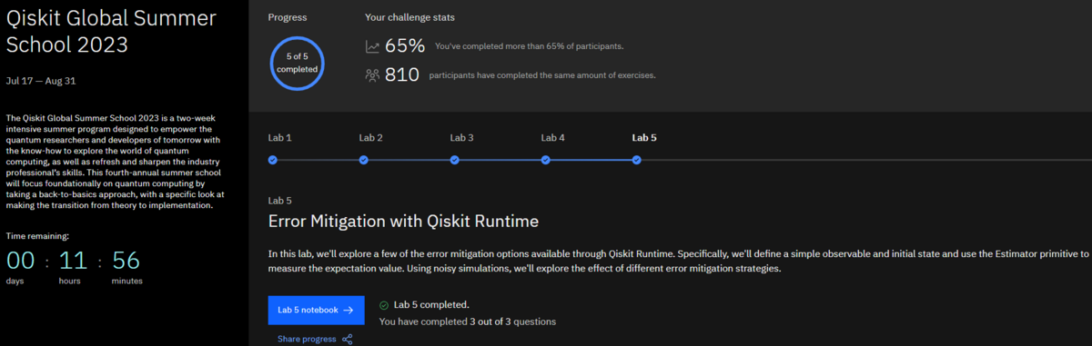
終了時のスクショ↓
各Labの記録
考察兼メモ代わりに記事を書きながら各Labを解いていきました。回答の解説っぽいものもあります。
- Lab1:記事なし。かなり基礎的な内容だった気がするので
- Lab2:Qiskit Global Summer School 2023 Lab2 参加記録
- Lab3:Qiskit Global Summer School 2023 Lab3 参加記録
- Lab4:Qiskit Global Summer School 2023 Lab4 参加記録
- Lab5:Qiskit Global Summer School 2023 Lab5 参加記録
