ABC292 E - Transitivity のTLE解
概要
ABC292 E - Transitivity の解法で、辺を管理するデータ構造をsetにするとTLEした。
setをforでアクセスするとTLEすることはあったが、count() や insert() の 対数時間でTLEしたのは初めて。
解法とコード
「既存の辺(u,v)をすべてdequeに突っ込む。dequeから辺(u,v)を取り出し、辺(v,w)のうちまだ(u,w)に辺が無いなら、dequeに(u,w)を追加して答えを+1する。dequeが空になるまで繰り返す」という解き方をした。
辺を管理するデータをg[i][j] := iからjへ辺があるとする。
ここで辺を管理するデータ構造をset<pair<ll,ll>> edgeSetにするとTLEするので注意。
bitsetを使えばもっと早い。
#include <bits/stdc++.h>
using namespace std;
using ll = long long;

void solve() {
    ll N, M; cin >> N >> M;
    vector G(N, vector<ll>());
    // set<pair<ll,ll>> edgeSet; // TLE
    // vector<bitset<2000>> g(N); // g[i][j] := iからjへ辺がある // AC
    vector g(N, vector(N, false)); // g[i][j] := iからjへ辺がある // AC
    deque<pair<ll,ll>> deq; // (u,v)
    for(ll i=0; i<M; i++) {
        ll u, v; cin >> u >> v;
        u--; v--;
        G[u].push_back(v);
        // edgeSet.insert({u,v});
        // g[u].set(v, 1);
        g[u][v] = true;
        deq.push_back({u,v});
    }

    ll ans = 0;
    while(!deq.empty()) {
        auto[u, v] = deq.front(); deq.pop_front();

        // vからwへの辺があるとき、uからwへの辺はあるか?
        for(ll w: G[v]) {
            if (u == w) continue;
            // if (!edgeSet.count({u,w})) {
            if (!g[u][w]) {
                // edgeSet.insert({u,w});
                // g[u].set(w, 1);
                g[u][w] = true;
                ans++;
                deq.push_back({u,w});
            }
        }
    }
    cout << ans << endl;
}


int main() {
    solve();
    return 0;
}
std::coutが正常に動作しない現象
概要
- 環境
- Windows10 64bit
- Powershell PSVersion 7.4.6
- g++.exe (Rev1, Built by MSYS2 project) 14.2.0
現象発生
std::coutが正常に動作しない現象(何も出力せずプログラムが強制終了)が発生しました。
#include <iostream>

int main() {
    printf("Hello World!\n"); // これは普通に出力される
    // std::ios::sync_with_stdio(false); // これを追加したらcoutできるようになる
    std::cout << "Hello World!!" << std::endl;  // 出力されない(プログラムが強制終了される)
    return 0;
}

コンパイルは正常にできているが、実行で赤くなっていることから、なにかしらのランタイムエラーが発生して落ちてしまっています。
不思議なのは、std::ios::sync_with_stdio(false);を追加すると正常に出力されるというところ。
調べると同様の現象っぽい人を見つけましたが、よくわかりませんでした。C++ stringを使用するとcoutが動作しない
行き詰まったので、ChatGPTに聞いてみます。

ターミナルの変更を勧められたのでGit Bashで試してみると、なんと実行結果が変わりました。

解決
これで検索すると、以下の記事を見つけました。
DLL地獄に引っかかってしまったようです。記事にあるようにコンパイルオプションに-static-libstdc++を追加すると、この現象は解消されました。

久しぶりに msys2 を再インストールしたら C:\msys64\bin が消えてた
タイトル通りなのですが、msys2.orgからmsys2-x86_64-20240727.exeをダウンロードし実行。WIndows10 64bit PCにインストールしました。
インストールガイドの言われるままにコマンドも実行。
$ pacman -S mingw-w64-ucrt-x86_64-gcc
インストール完了したあとにg++コマンドを打ってみてもそんなものは無いと言われるので、インストールフォルダを見に行ってみると、C:\msys64\binが消えてました。
どうやらMSYS2の構成が変わったらしく、clang64、mingw64、ucrt64などフォルダごとにbinが作られることになったらしいです。
色々調べましたが、なんかMS的にUCRTがおすすめっぽいので、とりあえずこちらを使ってみることにしました。
環境変数の設定にC:\msys64\ucrt64\binを追加し、VSCodeの設定ファイルも修正して終了。
gdb.exeも存在しなかったので、C++ Why is MSYS2 MINGW UCRT x64 gdb command not found - Stack Overflowを参考にインストールしました。
Causera: Generative AI for Software Development 感想
概要
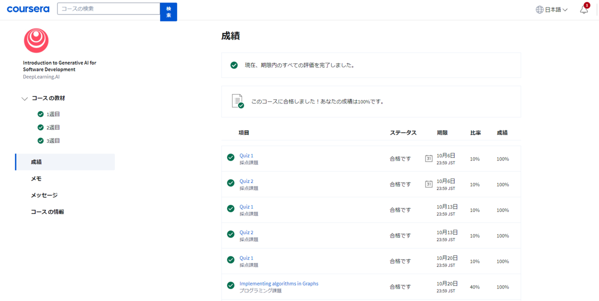
CauseraのGenerative AI for Software Developmentという講義が無料アクセスできたのでやりました。
この講義を受けた動機は、無料であったこと、Andrew Ngさんが講義に出ていること(実際はAndrewが出ているのはセクションの合間合間で、講義自体はLaurenceという方がする)、なんか良い良い言われているChatGPTの恩恵をあまり感じられてなかったからです。
無料期間中にさっさとやってさっさと退会したので認定証はもらっていません。


どんな講義
「開発者向けはじめてのChatGPTの使い方」みたいな講義でした。SNS等どこかで聞いたようなハウツー話が多かったのですが、役に立ったなと感じたところもありました。
ほとんどは動画視聴の講義で、練習問題として出されるデータ構造は基本的なものなので、まとまった時間と集中力が続く人は1日か2日ですべての講義を終えることができると思います。私は3日かかりました。
なるほどなぁと思ったのは、ChatGPTにRole(役割)を割り当てると良いという話。 「私はPython初心者で、あなたは私のメンターです。先程書いた関数について動作を説明して下さい」 「あなたはソフトウェアアーキテクトかつセキュリティスペシャリストです。次のコードの脆弱性を見つけ、可能なら改善案を書いて下さい」 「あなたはPythonのオープンソースコントリビューターです。先程の関数を批評し、改善点を提案して下さい」「あなたはソフトウェア設計パラダイムの専門家です。新しく発足する〇〇するプロジェクトにおいて、どのような開発手法を取り入れることを考えますか」 などと書くと、ChatGPTは役割に応じて説明してくれるようになり、またその役割に特化した情報を返してくれるようになります。
このようなRole割り当てをうまくやるためには、センスや慣れ、専門知識が必要になるでしょう。そして繰り返しChatGPTとやり取りを行い、「まあいいでしょう」となるまでコードをブラッシュアップしていく。
残念ながらありがたいことにAIは万能ではなく強力な同僚であり、人の仕事はまだ残っているということでした。
このへんのChatGPTに対するセンスは形式知にしておいてもらえると普通にありがたいので、「Effective ChatGPT ~ChatGPTと共にコードを書くときにに聞くべき100のこと~」みたいな本があったら読んでみたいなと思いました。
あとは便利だなと思ったのは、プロジェクトの依存関係解消などにもChatGPTは使えるということ。古いコードベースは変更したくなくて、それに合った古いpandasとnumpyを使うような面倒な依存関係解消も「バージョン〇〇のnumpyに対してはどのpandasのバージョンを使えば良いの」とChatGPTに聞くと答えてくれました。
このような話はYouTubeでも腐る程ありそうでCauseraに認定証料金7000円払う価値があるのかわからない――と思いましたが、腐る程ある動画を自発的に見る気は起きないので、その見る気を7000円で買えると考えればいいのではないでしょうか。あるいは、Laurenceにスーパーチャットを送ったという感覚で納得できるかもしれません。Laurenceの懐に入るかは知らないけれど。
感想
ChatGPTと共にコードを書くというのをあまりやってきてなかったので、結構新鮮な体験でした。今回ChatGPT-4oを使いましたが、「Copilotのない開発は考えられない」みたいなことを言う人の気持ちがすこしわかった気がしました。なるほど、これは良いものですね。
AHC026 参加記録
トヨタ自動車プログラミングコンテスト2023#6(AtCoder Heuristic Contest 026)に参加した記録です。
方針1:貪欲法
4時間の短期間コンテストなので、まずは正の得点を得られる簡単な貪欲ができないかを優先した。
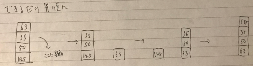
とりあえずビジュアライザを動かしてみて、どういう貪欲法がいいかを考える。
ターゲットの箱より上のすべての箱を、最も使わなそうな山を選んで、そこに積んでいく貪欲法をした。
「最も使わなそうな山」は、ターゲットの箱となるものが時間的に最も遠い山を選んだ。

提出コード:https://atcoder.jp/contests/ahc026/submissions/47302082
得点:1,356,657
この得点の人が多かったので、似たような解法をやってる人多そう。
方針2:ソートする?
箱を動かす時、なるべく上から昇順になるようにしたほうが、同じ体力で効率よく動かせるのでは?
結果的に言えば、重さ+1の体力を消費するのでそんなことなかった。
提出コード:https://atcoder.jp/contests/ahc026/submissions/47305951
得点:1,324,254
得点下がっちゃった。
方針3:ビームサーチ
多様性が確保できそうなのでビームサーチいけるかなと思って実装。永遠にバグらせて終了。
最終結果
方針1のコードが最終提出になった。
得点:1,356,657
順位:426位
強い人の方針
同じ色を集めてワーッてやって 70 位くらいでした #AHC026 pic.twitter.com/IHzgovj3sq
— iwashi31 (@iwashi31) 2023年11月5日
「片方に集める」「寄せる」みたいなのはAHCの典型なので最初そうしようかなと思ったのだけど、後半すっかり忘れていた。
#AHC026 1 位でした
— 和解 (@rsat__m) 2023年11月5日
各列について「全部の箱を別の列に出す」「sorted な状態で元の列に帰す」を行う方針を基本として、帰るときに出した先の箱もいい感じにくっつけて連れて帰ったり、既に sorted な列に出した分で帰ってこなくてもいいものを考慮したりするとじわじわスコアが改善する pic.twitter.com/TEvBTH0UO3
山が10個あるからうまくソート状態を作ればいいのか?(ハノイの塔のイメージ?)
感想
- 最初の貪欲の方針は悪くなかったと思う。
- ビームサーチバグらせたのは残念。実装方法のテンプレートをNotionにまとめておこう。
- でもビームサーチあんまりよいスコアでないらしい
- AHC楽しいので毎週開催してほしい。
- レートが単調増加は嬉しい。
AHC025 参加記録
概要
AtCoder Heuristic Contest 025に参加した記録です。
珍しいインタラクション問題。
方針1:ナイーブ実装
とりあえずシンプルな解法を考えて実装するところから着手した。以下のような解法になる。
- 最初、各グループは1つずつアイテムを持つ。残ったアイテムはすべてグループ0が持つ。
- s=0とする。
- グループsが他のグループに順番に1個ずつアイテムをランダムに渡していく。
- グループsがグループiにアイテムを渡したとき、グループiがグループsより重さが大きくなったら、s = iになって、再度3を繰り返す。
実装上の注意点として、
- アイテムが0個のグループを作ってはいけない
- 他のどのアイテムを足し合わせても敵わないような激重アイテムが1個ある場合、そのアイテム1個を唯一持つグループが出来上がる。このグループからその激重アイテムを取るとアイテムが0個になってしまうので取ってはいけない。
提出コード:https://atcoder.jp/contests/ahc025/submissions/46658987
得点:1,163,992,256
方針2:クイックソート実装
方針1の問題点は、「アイテムを1個ランダムに選んで渡す」とき、重いアイテムを渡す可能性があることにある。できれば軽いアイテムをやりとりして各グループの重さがならされるようにしたい。
ここで、クエリに2つのアイテムの大小関係を尋ねまくると、(アイテムの重さは不明のままだが)いずれアイテムをソートできることに気づく。アイテムがソートできた状態になると、各グループの一番軽いアイテムがわかるので、軽いアイテムを選択してやりとりすることで微調整できるようになる。
実装上の注意点として、
- クイックソートは最悪クエリ回数が(N-1)N/2 回かかる
提出コード:https://atcoder.jp/contests/ahc025/submissions/46693668
得点:811,781,427
今回の問題は得点が小さいほど良いスコアとなるので、改善されたと言える。
方針3:クイックソート打ち切り
方針2の改良。クイックソートに使えるクエリ回数上限を設定できるようにして、上限に達したら途中でソートを打ち切る。打ち切ると順番が中途半端にわからないアイテムがあるが気にしない。
アイテムの交換に使える最低クエリ回数を D*3 くらい(各グループ3回くらいアイテムのやりとりをするくらい)は確実に残すようにして、あとはクイックソートに使えるように設定した。もちろんクイックソートが早く終わればアイテムの交換に使えるクエリ回数は増える。
これにより方針1のナイーブ実装の実行を完全に排除できた。(運次第だと思うが、ナイーブ実装のほうが良いスコアのサンプルがちらほらあったが……)
提出コード:https://atcoder.jp/contests/ahc025/submissions/46697190
得点:586,051,759
このあと、アイテムの交換に使える最低クエリ回数の値をいろいろ試したところ、D*5 が最もスコアが良かったので最終的にそうした。
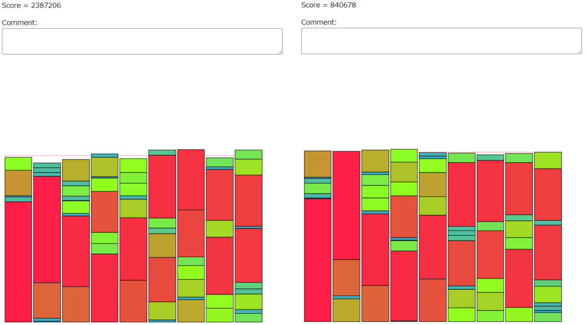
方針4:グループの重さのクイックソート実装
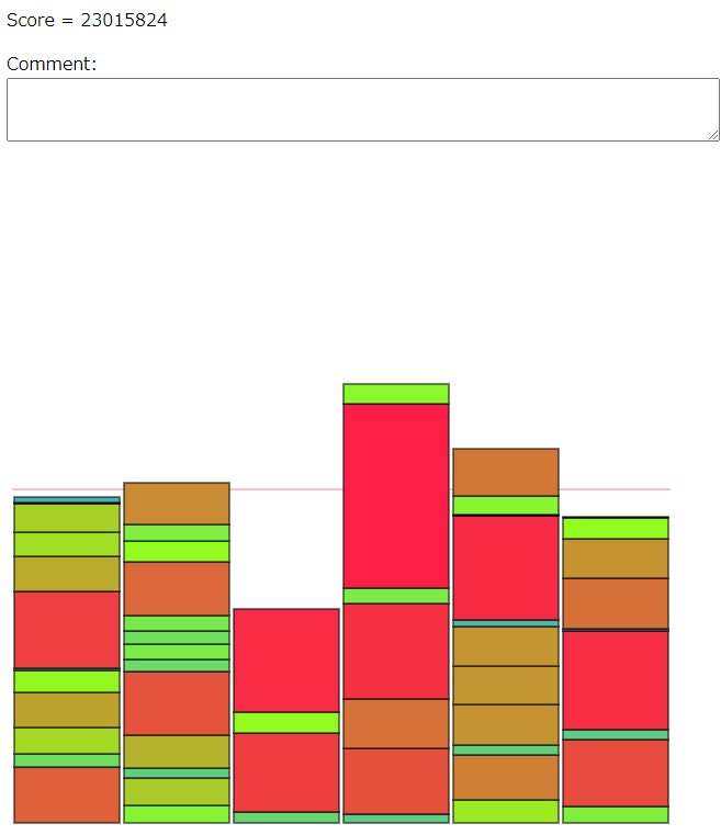
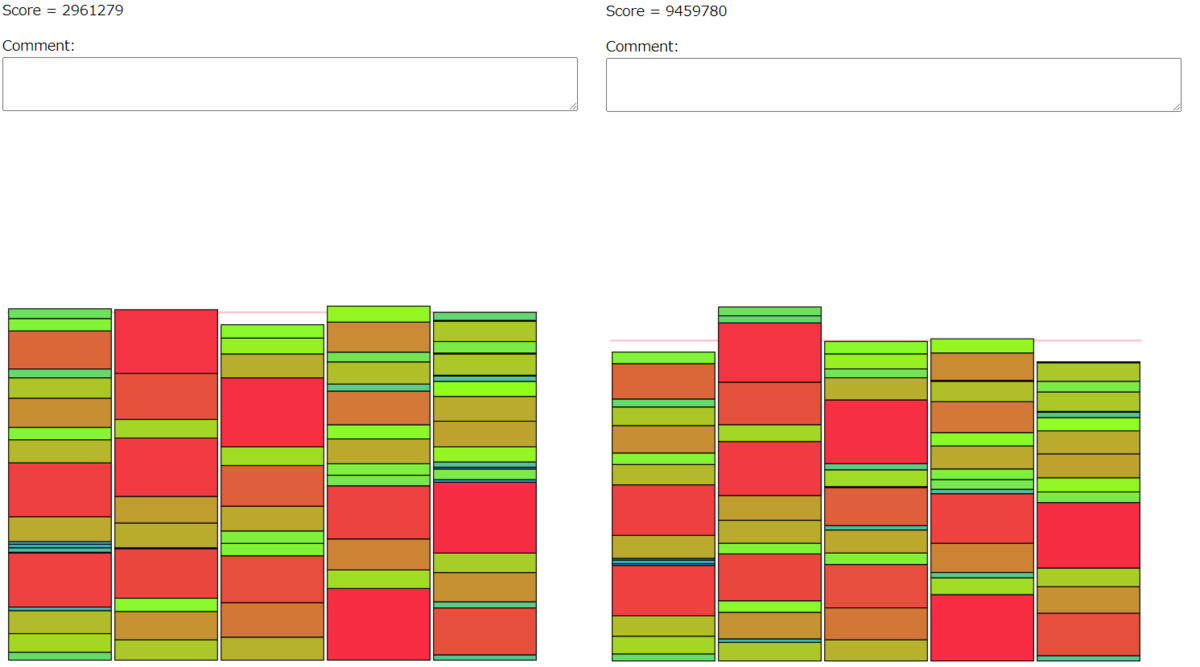
Seed 29を考察した。
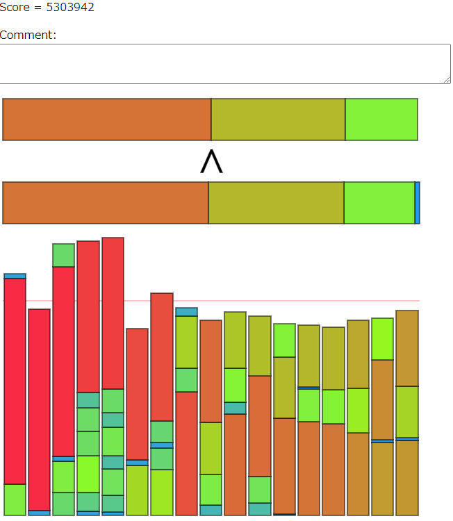
シード29は完全にソートされているにも関わらず、あまり良くないスコアになっている。
たとえば、左から5番目のグループは軽いアイテムをたくさん持っているにも関わらず、それらを貯め込んで一番重いグループになっている。こいつのグループが他のグループに軽いアイテムを配ってくれればもっと良いスコアになるはず。
分析の結果、全1423ターンのうち、509ターン目でソートが完了し、残り約900 ターンでアイテム交換をしていた。アイテム交換に十分のターン数があるにも関わらず、スコアは良くない結果になっている。
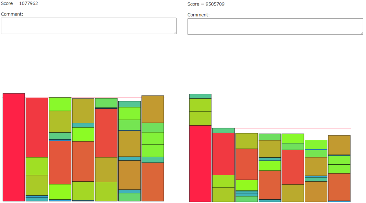
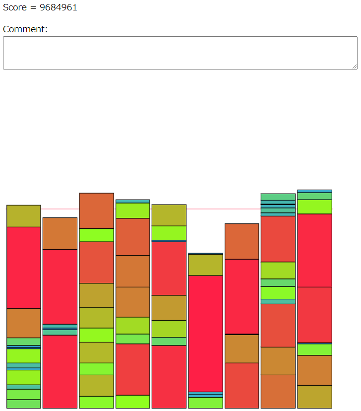
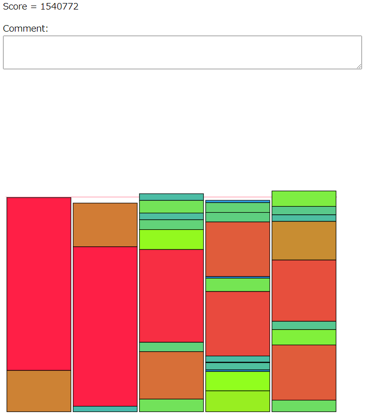
もっと深く考察するために、途中結果を出力して確認してみる。
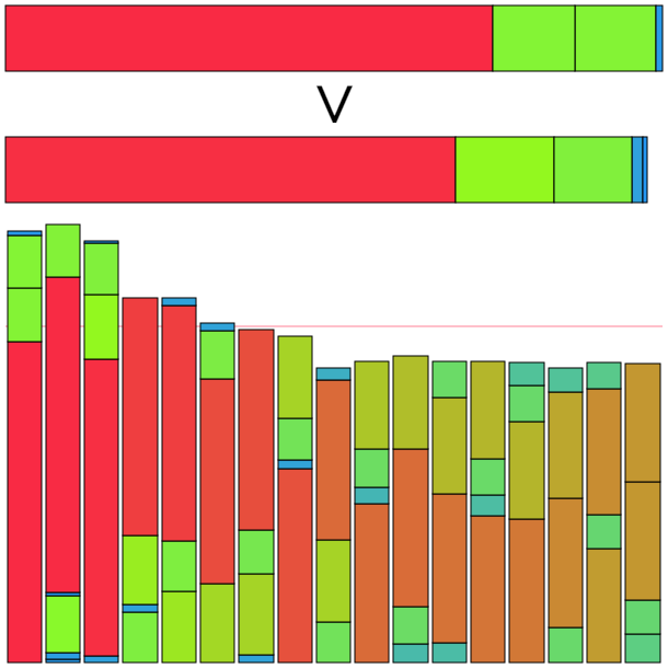
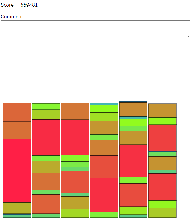
ソート完了直後は上の状態となった。
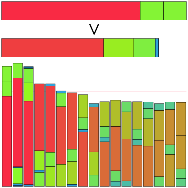
一番左と、左から3番目のアイテムの交換が行われた。
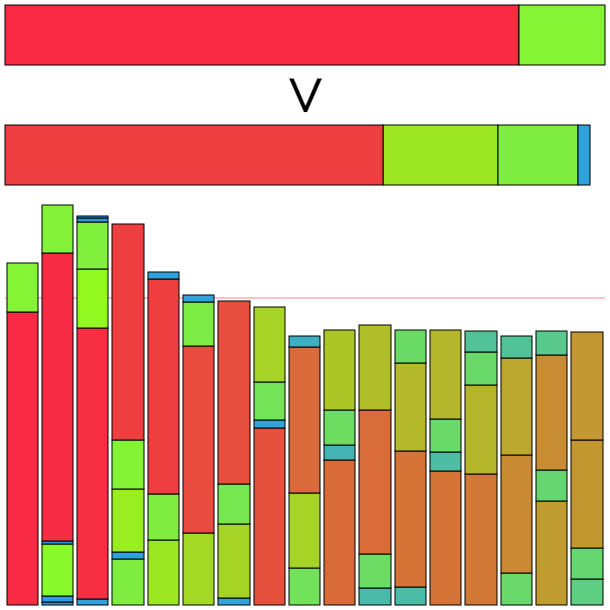
一番左と、左から4番目のアイテムの交換が行われた。
これを見ると、重いグループ同士で無駄な交換が起きているように見える。なので、クエリ回数が十分に残っている場合(最悪交換回数の(D-1)*D/2以上の場合)、各グループの重さでソートし、「重いグループと軽いグループで交換を行う」ということをすれば良さそうである。
すなわち今回の方針では、グループの重さのクイックソートを実装した。
提出コード:https://atcoder.jp/contests/ahc025/submissions/46748553
得点:602,827,302
スコアが悪くなってしまった。
方針5:方針4の改良(残りクエリ回数を十分取るときだけグループのソートをする)
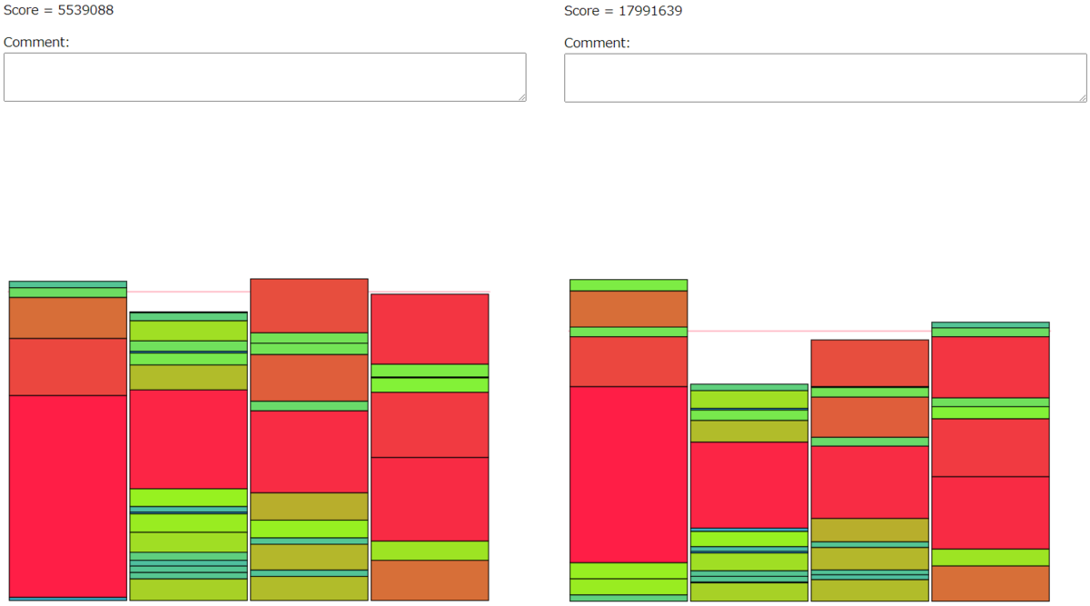
方針4では、残りクエリ回数が十分にあるときだけグループのクイックソートをして、そうでないときは方針3に切り替えるように調整した。それでもスコアが悪かったので、何がいけないのか出力ファイルを比較して原因を探った。
悪くなったサンプルを比較してみる。
以下の分数は、(アイテムのソートで使ったクエリ回数)/(全クエリ回数)。
シード7の比較。
278/294
シード8の比較。
175/197
シード16の比較。
206/221
良くなったサンプルを比較してみる。
シード1の比較。
306/1120
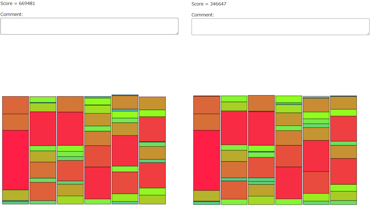
シード18の比較。
368/1028
他にも比較したが割愛。
比較してわかったのが、 (アイテムのソートで使ったクエリ回数)/(全クエリ回数)の値が大きい (=アイテムのソート後に残ったクエリ回数が少ない)と、グループのソートに使えるクエリ回数が少なすぎて方針3より悪いスコアになってしまうらしいということ。
つまり残りクエリ回数が十分にあるときだけグループのクイックソートをしていたつもりが、まだまだ全然足りなかったということらしい。
残りクエリ回数がQ/2以上のときだけグループのクイックソートをするように変更した。
提出コード:https://atcoder.jp/contests/ahc025/submissions/46748977
得点:543,035,466
方針3よりスコアが良くなった。
上記の方針5では、方針3よりサンプル100個中、
- 5個スコアが悪くなった
- 31個スコアが改善された
- 64個はスコアが変わらなかった
方針6:残りクエリ回数に応じて確率的にグループの重さが切り替わるようなアイテム交換を許す
方針5では、64個はスコアが変わらないのであった。これは、アイテムのソート後に残りクエリ回数が少ないので方針3に切り替わった個数が64個ということであった。
方針3の問題点はなんだろうかと、いくつか悪いスコアのものをピックアップしてみた。
seed62: 157/185

seed66: 438/482
ビジュアライザを動かしてみると、残りクエリ回数が少ないときにもグループ間の重さが入れ替わるような重いアイテムの交換を許してしまっていた。
残りクエリ回数がまだ残ってるときはグループの重さが入れ替わってもいいが、残りクエリ回数が少ないときはグループの重さが入れ替わるようなことはせず、軽いアイテムのやりとりだけで済ましてほしい。イメージ的には『安定』したやりとりをしてほしいという欲求がある。
なので、残りクエリ回数に応じて確率的にグループの重さが切り替わるようなアイテム交換を許す実装をした。気持ち的には焼き鈍し法である。

かなり良くなった感じがしたので、提出した。
提出コード:https://atcoder.jp/contests/ahc025/submissions/46841307
得点:492,973,943
最終結果
方針6を最終結果として提出した。
A:58,654,377,877
A-Final:300,672,027,666
順位:458
ここまでの感想
- 方針5を実装した時点での相対スコアが62Gで、順位は380位くらいだった。この得点帯は激戦区で、寝て起きたら順位が結構下がっている。
- 方針5を実装した時点で頭打ちしてると思ったのだが、上位陣が90Gで途方もなかった
- 「山登り、焼きなまし、ビームサーチは絶対にできないよな」「いやしかし…」とぐるぐる考えてた
- 方針6は発想としてはかなり焼き鈍し法なのだが、これに至るまでかなり時間を要した。
公式解説
X(Twitter)で調べると強い人はソートして一番重いものと一番軽いものを交換している人が多いイメージ。似たようなことは自分もしているのだが、自分の解法では一番重いやつと軽いやつを交換、2番目に重いやつと軽いやつを交換、…としていたのが良くなかったのか?
公式解説の動画を見てみる。
- 解法1:クエリを使ってがんばって重さを推測する。その後クエリを使わずに最適化問題を解く
- 解法2:焼きなまし法(近傍解を求めて、その近傍解が良くなったら採用。悪くなったら悪くなった度合いに応じて確率的に採用)は、今回の天秤を使ったクエリでは「どれだけ悪くなった」かがわからないので難しい(「悪くなった」はわかるが「どれだけ悪くなったか」はわからない)。が、「良くなった」のは判定できるので、山登り法が可能
- 初期解を適当に作って、山登り法をする
- 解法3:初期解を貪欲法で作る
公式解説では解法2の山登りを解説してくれた。
山登り法
2つのグループの大小関係がわかっている状態で、アイテム交換をする。アイテム交換後、2つのグループの大小関係が変わっていなかったら、「スコアが良くなった」といえる(2つのグループ間の分散が小さくなっているので)。
基本的にはこれをひたすら山登っていけばいい。
この解法のシンプルな手法ではソートすら必要なくて、アイテムをランダムに1個選び、それをどこのグループに入れるかもランダムに選ぶ。アイテム交換してスコアが良くなるなら交換し、スコアが良くならないなら交換しない。
初期解は各グループ同じアイテムの個数になるように適当に割り振る。
これをすると321位がとれるらしい。
うーーーーーーーーーん。シンプルな解法に見えるが、これでも十分自分より良い点数が取れるところを見ると、考察力が足りないと感じる。やってることは「言われてみれば当然といえば当然」のことなのだが、思いついてないんだよなぁ。
アイテム交換方法2
もうひとつのアイテム交換方法として、グループAとグループBからそれぞれアイテムを1個ずつ取り出して、取り出したアイテムをアイテムa、アイテムbとする。
このとき、「グループA < グループB」「アイテムa < アイテムb」ならば、アイテムaはグループBに入れ、アイテムbはグループAに入れるとスコアが良くなる。
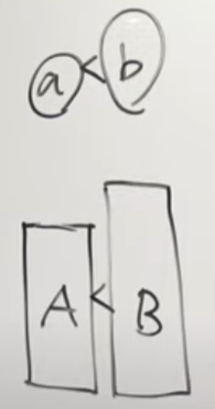
このようなアイテム交換はクエリ2回の発行で行える。
「この交換法も50%の確率でする」みたいに組み合わせると218位に入れるらしい。
キャッシュする + 推移律のグラフを作る
一度した交換方法はキャッシュして覚えて、2回もしないようにすると地味に良くなる。
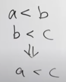
アイテム交換方法2をすると、アイテムの大小関係のデータが蓄積していく。
a < b のような大小関係のグラフを作っておくと、a < b と b < c => a < c のように、クエリを発行しなくても推移律で新たに大小関係が判明する。
もっとやろうと思えば以下のように導くこともできる。
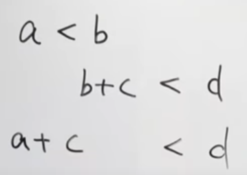
こういう不等式系がたくさんあったときにすべて満たす解を求める方法にLP(線形計画法)があるらしい。
それをしなくても「アイテムa+cとアイテムdの交換」といった複数個の交換が可能になる。
これを実装すると200位になる。
グループのソートを実装する
これまでの方法の問題点は、交換するグループをランダムに選んでいたのが問題であった。
そこでグループのソートを実装すると、どのグループがアイテムを交換すべきなのかがわかる。
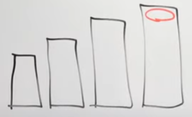
アイテム交換後のグループのソートは単純にやればO(DlogD)。けどこれは以下のようにして改善できる。
一番重いグループをグループA、一番軽いグループをグループBとする。アイテム交換後、グループAとグループB以外の他のグループはソート済みなので、「グループA(B)は、ソート済みのグループのどこに入るか」を2分探索すればO(logD)で済む。確かに……。
これをすると49位になる。
公式解説の感想
- 公式解説を見ると、「なぜこれが思いつかなかったのか……」といった感想になった。ソートなどそれっぽいことは思いついて実装できているのだが、初期の解法の土台が良くないのでスコアが伸びなかった印象。論理的な道筋が見えていないのというか。練度が足りない。
AHC024 参加記録
概要
丸紅プログラミングコンテスト2023(AtCoder Heuristic Contest 024)に参加しました。4時間の短期間コンテストでした。
ほぼ何もできなかったといってもいい。
最初の方針
連結成分をノード、「隣接する」というのを辺と考えるとグラフができるので、そのグラフからグリッドを作ろうと思いましたが、実装が大変で2時間経過。スジが悪いと思い直してビジュアライザをいじっていると、与えられたグリッドを白に塗っていくのほうが実装が簡単なことに気づきました。
かなりバグ散らかしつつ終了10分前くらいにかなりナイーブな貪欲ができたのでそれを提出。終了です。
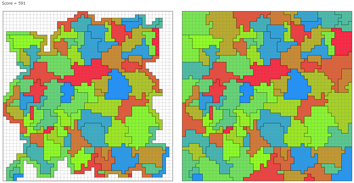
白に塗れるところは貪欲に白に塗っていく。
真ん中あたりのエリアが大きいですね。これらを隣接条件等を崩さないように圧縮していければなあと思いつつ終了しました。あと4時間ほしい。
上手い人の解法
#AHC024
— ゴジラ@競プロ (@gojira_kyopro) 2023年9月24日
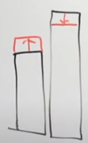
seed=0 で 1996 点
中心に向かって縮める感じで pic.twitter.com/eQTnDwj8wW
中心に寄せる貪欲らしいです。貪欲でもここまでいけるらしい。
https://twitter.com/Jiro_tech15/status/1705889677910348053
左上に寄せていき、最後にぎゅっと圧縮する手法。おお、と思いました。AHC系は「はしっこに寄せる」という発想はよく見る気がします。
アニメーション機能を使って可視化してみました #AHC024 #丸紅 https://t.co/ACJ86sOuHc pic.twitter.com/8ysGQfQg0O
— ymatsux (@ymatsux_ac) 2023年9月24日
消せる行や列を消すという発想。「隣接条件を崩さずにどう圧縮するか」というのを考えたとき、たしかに「1行ごっそり消せるなら消す」というのは実装ラクそう。天才や……
反省
AHCやることメモに「まずビジュアライザをいじる」って書いてあるだろ。なぜそれをしないんだ。
短時間コンテストは実装のしやすさ・速さがかなり重要だと感じました。
あと最近、C++でクラスを書くときはメンバ変数にm_のプレフィックスをつけているのだがいい感じ。メンバにアクセスするときは通常this->を使うと思うのだが、長いのがやだ。