各Labの記録

参加結果の記事：Qiskit Global Summer School 2023 参加記録
Lab1：記事なし。かなり基礎的な内容だった気がするので
Lab2：Qiskit Global Summer School 2023 Lab2 参加記録
Lab3：Qiskit Global Summer School 2023 Lab3 参加記録
Lab4：Qiskit Global Summer School 2023 Lab4 参加記録
Lab5：Qiskit Global Summer School 2023 Lab5 参加記録

まえがき

Qiskit Global Summer School 2023 Lab3の記録です。

Lab 3 : Diving Into Quantum Algorithms

ex1

5量子ビット（位相推定用のビット数4 + 補助量子ビット数1個）のQPE回路を作る問題。以下の回路を作れば良い。

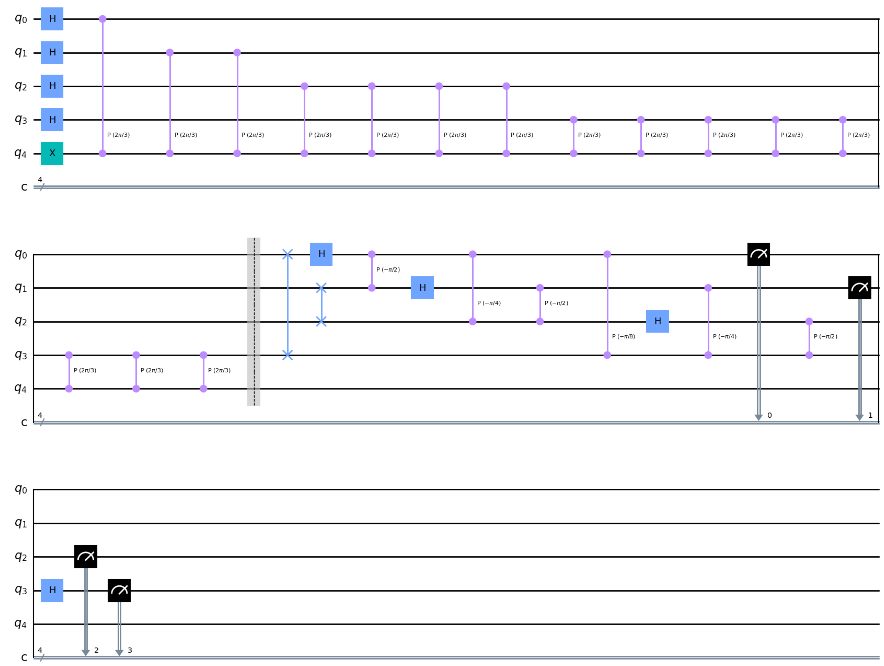
QFTと逆QFTのサンプルコードは与えられているので、それらを使って作ることができる。

#QFT Circuit
def qft(n):
    """Creates an n-qubit QFT circuit"""
    circuit = QuantumCircuit(n)
    def swap_registers(circuit, n):
        for qubit in range(n//2):
            circuit.swap(qubit, n-qubit-1)
        return circuit
    def qft_rotations(circuit, n):
        """Performs qft on the first n qubits in circuit (without swaps)"""
        if n == 0:
            return circuit
        n -= 1
        circuit.h(n)
        for qubit in range(n):
            circuit.cp(np.pi/2**(n-qubit), qubit, n)
        qft_rotations(circuit, n)
    
    qft_rotations(circuit, n)
    swap_registers(circuit, n)
    return circuit

#Inverse Quantum Fourier Transform
def qft_dagger(qc, n):
    """n-qubit QFTdagger the first n qubits in circ"""
    # Don't forget the Swaps!
    for qubit in range(n//2):
        qc.swap(qubit, n-qubit-1)
    for j in range(n):
        for m in range(j):
            qc.cp(-np.pi/float(2**(j-m)), m, j)
        qc.h(j)
    return qc

phase_register_size = 4
qpe4 = QuantumCircuit(phase_register_size+1, phase_register_size)

### Insert your code here
# Preparation
for i in range(4):
    qpe4.h(i)
qpe4.x(4)

# Apply CP Gate
angle = np.pi*2/3 # λ
for i in range(4):
    for _ in range(2**i):
        qpe4.cp(angle, i, 4)
qpe4.barrier()

# Apply QFT^dagger
qpe4 = qft_dagger(qpe4, 4)

# Measure
for i in range(0, 4):
    qpe4.measure(i, i)

qpe4.draw()

シミュレータ実行すると以下が得られた。

## Run this cell to simulate 'qpe4' and to plot the histogram of the result
sim = Aer.get_backend('aer_simulator')
shots = 2000
count_qpe4 = execute(qpe4, sim, shots=shots).result().get_counts()
plot_histogram(count_qpe4, figsize=(9,5))

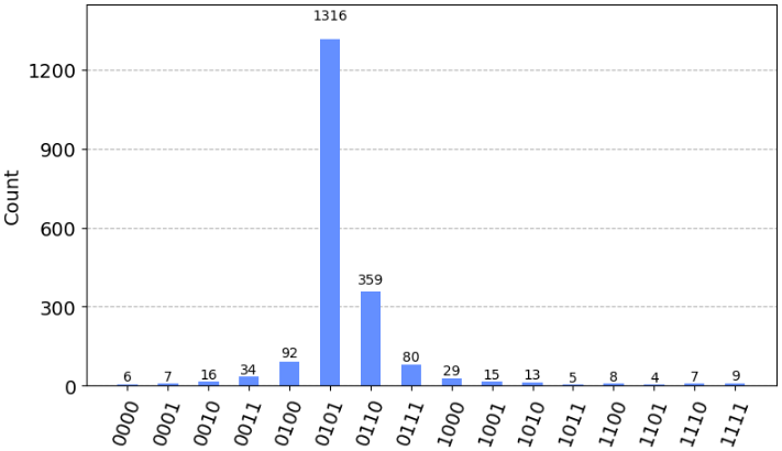
結果は 0101 が最も大きい確率となった。

位相推定の結果 $\theta_{e}$ は、

N: 最も確率が高かった値（10進数）
n: 位相推定用のビット数

とすると、 $\theta_{e} = \frac{N}{2^{n}}$ で求めることができる。詳しくはSampler primitive を使用した量子位相推定に書いてある。

2進数の 0101 は10進数で 5 なので位相推定の結果は、

estimated_phase = 5/(2**phase_register_size)
print("estimated_phase: ", estimated_phase)
print("誤差: ", abs(estimated_phase - 1/3))
# estimated_phase:  0.3125
# 誤差:  0.020833333333333315

となる。たしかに真値θ = 1/3 (=0.3333...) に近い値を推定できたということになる。

余談だが、今の状態で更に精度を上げるにはSampler primitive を使用した量子位相推定#ステップ-3:-結果の分析に書いてあるように、2番目に確率が大きい値との加重平均を取ればいい（最も確率が大きい値の近傍になっていることが望ましい）。

今回の場合で言えば2番目に確率が大きいのは 0110 (10進数で6)であり、最も確率が高い5の近傍であるので適している。加重平均をとった結果は以下になる。

# 2番目に確率が大きい値との加重平均をとると更に良さそう
estimated_phase1 = 5/(2**phase_register_size)
estimated_phase2 = 6/(2**phase_register_size)
estimated_phase = (estimated_phase1+estimated_phase2)/2
print("estimated_phase: ", estimated_phase)
print("誤差: ", abs(estimated_phase - 1/3))
# estimated_phase:  0.34375
# 誤差:  0.010416666666666685

簡単に真値θ = 1/3 (=0.3333...)との誤差を小さくすることができた。

ex2

位相推定の結果は何？
この回路は最大で2の何乗までの精度を計算できるか？

の2つを答える問題。2番目の答えの意味を汲むのが少しむずかしかった。

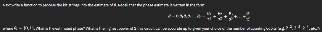
今回位相推定用のビット数tは4なので、 $\frac{1}{2^{4}}$ までの精度を計算できる。

#Grab the highest probability measurement
max_binary_counts = 0
max_binary_val = ''
for key, item in count_qpe4.items():
    if item > max_binary_counts:
        max_binary_counts = item
        max_binary_val = key

## Your function to convert a binary string to decimal goes here
# calculate the estimated phase
dec = 0
for i, c in enumerate(max_binary_val[::-1]):
    dec += (2**i) * int(c)
estimated_phase = dec/(2**phase_register_size)
print("estimated_phase: ", estimated_phase)

# highest power of 2 (i.e. smallest decimal) this circuit can estimate
phase_accuracy_window = 1/(2**4)
print("phase_accuracy_window: ", phase_accuracy_window)

ex3

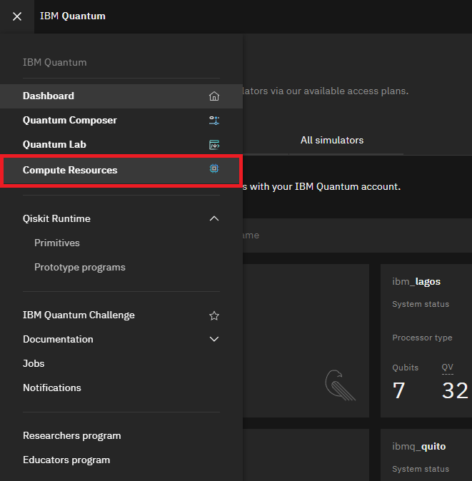
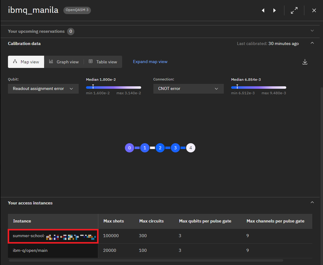
実機情報を得るために provider_get_backend() する必要があるのだが、引数に渡す hub, group, project がなんなのか分からなくて困った。Discordに書いてあった。

For the hub, group, and project, From main page menu of IBM Quantum Experience portal -> Computer Resources - > Your Resources ( Select Table view from right)- > click on ibmq_manila -> go to the section Your Access Instance -> Details will be in a string of format summer-school-x/group-x/xxxxxxxxxx

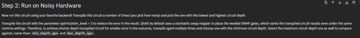
IBM Quantum Experience portal -> Computer Resources

Qiskitはデフォルトで確率的スワップマッパーを使用して必要なSWAPゲートを配置するため、同じランタイム設定であってもトランスパイルされた回路結果にばらつきが生じる。回路深度の短いトランスパイル回路の方が結果の誤差は小さくなるので、qpe4を複数回トランスパイルして回路深度が最小のものを選ぶ必要がある。

transpile方法は qiskit.compiler.transpile に書いてある。

from qiskit_ibm_provider import IBMProvider
from qiskit.compiler import transpile

# summer-school-x/group-x/xxxxxxxxxx
provider = IBMProvider()
hub = "summer-school-x"
group = "group-x"
project = "xxxxxxxxxx"
backend_name = "ibmq_manila"

backend = provider.get_backend(backend_name, instance=f"{hub}/{group}/{project}")

# your code goes here
# 適当に100回トランスパイルして、最も深い回路と最も浅い回路をそれぞれ得る
max_depth = 0
min_depth = 999
min_depth_qpe = None
max_depth_qpe = None
for _ in range(100):
    transpiled_qc = transpile(circuits=qpe4, backend=backend, optimization_level=3)
    if transpiled_qc.depth() > max_depth:
        max_depth = transpiled_qc.depth()
        max_depth_qpe = transpiled_qc
    if transpiled_qc.depth() < min_depth:
        min_depth = transpiled_qc.depth()
        min_depth_qpe = transpiled_qc

print("min_depth_qpe.depth(): ", min_depth_qpe.depth())
print("max_depth_qpe.depth(): ", max_depth_qpe.depth())
# min_depth_qpe.depth():  75
# max_depth_qpe.depth():  78

最も浅い回路を実行してみる。

shots = 2000

#OPTIONAL: Run the minimum depth qpe circuit
job_min_qpe4 = backend.run(min_depth_qpe, sim, shots=shots)
print(job_min_qpe4.job_id())

#Gather the count data
count_min_qpe4 = job_min_qpe4.result().get_counts()
plot_histogram(count_min_qpe4, figsize=(9,5))

cj6rcddtks61ugsn95hg
Traceback (most recent call last):
  Cell In[86], line 8
    count_min_qpe4 = job_min_qpe4.result().get_counts()
  File /opt/conda/lib/python3.10/site-packages/qiskit_ibm_provider/job/ibm_circuit_job.py:250 in result
    raise IBMJobFailureError(f"Job failed: " f"{error_message}")
IBMJobFailureError: 'Job failed: Internal Error while executing OpenQASM 3 circuit.'

Use %tb to get the full traceback.

なんかエラーが出て実行できなかったので、代わりにFakeManilaV2を使ったシミュレータ実行をした。

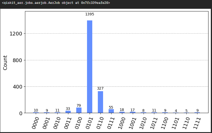
最も浅い回路の実行結果は以下になった。

# なんか実機のバックエンド実行でエラーが出たので、しょうがないのでシミュレータを使って実行する
from qiskit.providers.fake_provider import FakeManilaV2
backend_fakemanilav2 = FakeManilaV2()

shots = 2000

#OPTIONAL: Run the minimum depth qpe circuit
job_min_qpe4 = sim.run(min_depth_qpe, backend=backend_fakemanilav2, shots=shots)
print(job_min_qpe4.job_id())

#Gather the count data
print(job_min_qpe4)
count_min_qpe4 = job_min_qpe4.result().get_counts()
plot_histogram(count_min_qpe4, figsize=(9,5))

最も深い回路の実行結果は以下になった。

# こちらもシミュレータを使って実行する
job_max_qpe4 = sim.run(max_depth_qpe, backend=backend_fakemanilav2, shots=shots)
print(job_max_qpe4.job_id())

#Gather the count data
count_max_qpe4 = job_max_qpe4.result().get_counts()
plot_histogram(count_max_qpe4, figsize=(9,5))

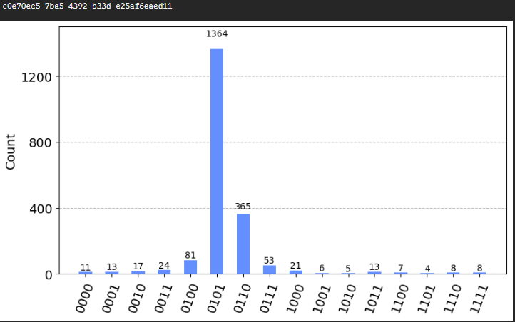
min_depth_qpeの方が0101の確率が高いので、（誤差の範疇の気もするが）たしかに精度が高いと言える。

ex4

「真値θ=1/7 としたときの位相推定をするとき、誤差が2^-6以下になるのに必要な最小の位相推定用のビット数は？」という問題。

位相推定用のビット数register_sizeを指定してQPE回路を作る関数は以下のようにする。

Pゲートのλの値はどうするか？

ちなみに「Pゲートのλの値を決めるためには推定すべきθの値を知ってないといけないのはどういうことやねん。意味あんのか？」という疑問はもっともである。この疑問は因数分解ソルバーであるショアのアルゴリズムが少し解消してくれる。

さらにちなみに、Qiskit Textbook の量子位相推定ではPゲートの代わりにTゲートを使っているが、考え方は同じである。

def qpe_circuit(register_size):
    # Your code goes here
    qpe = QuantumCircuit(register_size+1, register_size)

    # Preparation
    for i in range(register_size):
        qpe.h(i)
    qpe.x(register_size)

    # Apply CP Gate
    angle = np.pi*2/7 # λ
    for i in range(register_size):
        for _ in range(2**i):
            qpe.cp(angle, i, register_size)
    qpe.barrier()

    # Apply QFT^dagger
    qpe = qft_dagger(qpe, register_size)

    # Measure
    for i in range(0, register_size):
        qpe.measure(i, i)

    return qpe

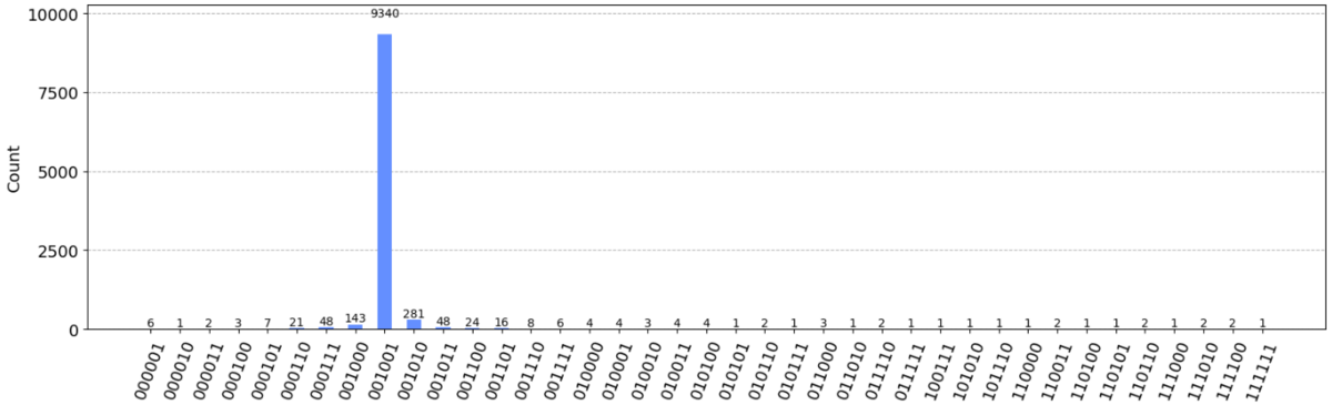
位相推定用のビット数 reg_size=6 としたときの結果は以下のようになった。

## Run this cell to simulate 'qpe4' and to plot the histogram of the result
reg_size = 6# Vary the register sizes

qpe_check = qpe_circuit(reg_size)
sim =  Aer.get_backend('aer_simulator')
shots = 10000
count_qpe4 = execute(qpe_check, sim, shots=shots).result().get_counts()
plot_histogram(count_qpe4, figsize=(19,5))

真値との誤差を計算する関数を以下のように作った。

# 真値との誤差を計算する関数
def calc_error(count_qpe):
    #Grab the highest probability measurement
    max_binary_counts = 0
    max_binary_val = ''
    for key, item in count_qpe.items():
        if item > max_binary_counts:
            max_binary_counts = item
            max_binary_val = key

    ## Your function to convert a binary string to decimal goes here
    # calculate the estimated phase
    dec = 0
    for i, c in enumerate(max_binary_val[::-1]):
        dec += (2**i) * int(c)
    estimated_phase = dec/(2**reg_size)
    print("estimated_phase: ", estimated_phase)

    # 真値
    true_phase = 1/7
    print("true phase: ", true_phase)

    # 誤差
    error = abs(estimated_phase-true_phase)
    print("誤差: ", error)
    
    return error

さて、誤差が2^-6以下となるような最小のビット数を求めたい。1から順に回して調べればよい。

# 誤差が2^-6以下になるために必要な最小のビット数は？
required_register_size = 1
for n in range(1, 100):
    print("===register_size:{}===".format(n))
    reg_size = n# Vary the register sizes

    qpe_check = qpe_circuit(reg_size)
    sim =  Aer.get_backend('aer_simulator')
    shots = 10000
    count_qpe = execute(qpe_check, sim, shots=shots).result().get_counts()
    
    error = calc_error(count_qpe)

    # 誤差が2^-6以下になったら終了
    if error <= 2**(-6):
        required_register_size = n
        break
print(required_register_size)

===register_size:1===
estimated_phase:  0.0
true phase:  0.14285714285714285
誤差:  0.14285714285714285
===register_size:2===
estimated_phase:  0.25
true phase:  0.14285714285714285
誤差:  0.10714285714285715
===register_size:3===
estimated_phase:  0.125
true phase:  0.14285714285714285
誤差:  0.01785714285714285
===register_size:4===
estimated_phase:  0.125
true phase:  0.14285714285714285
誤差:  0.01785714285714285
===register_size:5===
estimated_phase:  0.15625
true phase:  0.14285714285714285
誤差:  0.01339285714285715
5

ということで5が正解。

ex5

テーマはショアのアルゴリズムの実装に移る。

ショアのアルゴリズムのQiskitの記事が消えてて（検索してもいいのが出てこなかった）困ったのだが、素因数分解アルゴリズムを学習する — 量子コンピューティング・ワークブックの記事がわかりやすかったのでそれを参考にした。

さて、Uゲートとして「7mod15ゲート」を作ったので、それが正しく動作するかチェックしようという問題。

### your code goes here

# |1>で確認する
qcirc = QuantumCircuit(m)
qcirc.x(0)
qcirc.append(U, [i for i in range(m)])
qcirc.measure_all()
qcirc.draw()

# |2>で確認する
qcirc2 = QuantumCircuit(m)
qcirc2.x(1)
qcirc2.append(U, [i for i in range(m)])
qcirc2.measure_all()
qcirc2.draw()

# |5>で確認する
qcirc5 = QuantumCircuit(m)
qcirc5.x(0)
qcirc5.x(2)
qcirc5.append(U, [i for i in range(m)])
qcirc5.measure_all()
qcirc5.draw()

回答コードは以下。

## Run this cell to simulate 'qpe4' and to plot the histogram of the result
sim = Aer.get_backend('aer_simulator')
shots = 20000

input_1 = execute(qcirc, sim, shots=shots).result().get_counts()  # save the count data for input 1

input_2 = execute(qcirc2, sim, shots=shots).result().get_counts()# save the count data for input 2
input_5 = execute(qcirc5, sim, shots=shots).result().get_counts()# save the count data for input 5

input_1をヒストグラムで表示すると、以下になった。

plot_histogram(input_1, figsize=(10,5))

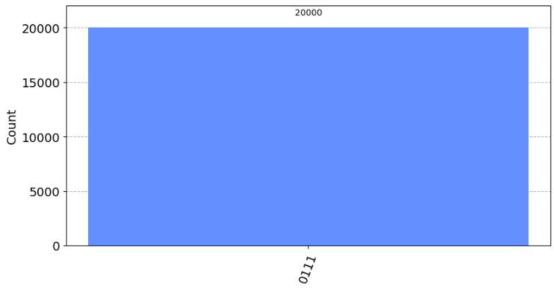
1*7 mod 15 ≡ 7(0111) なので、正しい結果が得られている。

他2つの結果も載せておく。どれも正しい結果が得られているので、正しく実装できたようだ。

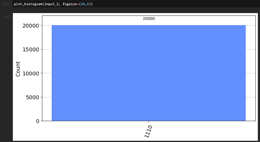
2*7 mod 15 ≡ 14(1110)

5*7 mod 15 ≡ 5(0101)

ex6

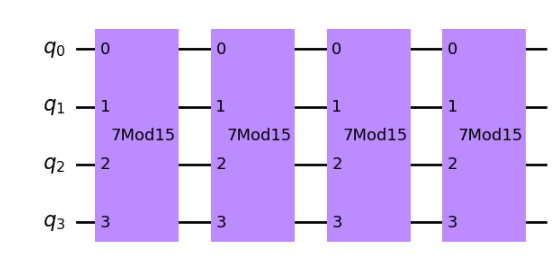
7mod15ゲートは4回適用するとIゲートと同じということを確認する問題。

たしかに、7 * 7 * 7 * 7 ≡ 1 (mod 15) なので、その通りである。

unitary_circ = QuantumCircuit(m)

# Your code goes here
for i in range(4):
    unitary_circ.append(U, [i for i in range(m)])

unitary_circ.draw()

回路を unitary_simulator で実行して、結果をユニタリ行列化したものを見てみよう。

sim = Aer.get_backend('unitary_simulator')
unitary = execute(unitary_circ, sim).result().get_unitary()
print(unitary)

Operator([[1.+0.j, 0.+0.j, 0.+0.j, 0.+0.j, 0.+0.j, 0.+0.j, 0.+0.j, 0.+0.j,
           0.+0.j, 0.+0.j, 0.+0.j, 0.+0.j, 0.+0.j, 0.+0.j, 0.+0.j, 0.+0.j],
          [0.+0.j, 1.+0.j, 0.+0.j, 0.+0.j, 0.+0.j, 0.+0.j, 0.+0.j, 0.+0.j,
           0.+0.j, 0.+0.j, 0.+0.j, 0.+0.j, 0.+0.j, 0.+0.j, 0.+0.j, 0.+0.j],
          [0.+0.j, 0.+0.j, 1.+0.j, 0.+0.j, 0.+0.j, 0.+0.j, 0.+0.j, 0.+0.j,
           0.+0.j, 0.+0.j, 0.+0.j, 0.+0.j, 0.+0.j, 0.+0.j, 0.+0.j, 0.+0.j],
          [0.+0.j, 0.+0.j, 0.+0.j, 1.+0.j, 0.+0.j, 0.+0.j, 0.+0.j, 0.+0.j,
           0.+0.j, 0.+0.j, 0.+0.j, 0.+0.j, 0.+0.j, 0.+0.j, 0.+0.j, 0.+0.j],
          [0.+0.j, 0.+0.j, 0.+0.j, 0.+0.j, 1.+0.j, 0.+0.j, 0.+0.j, 0.+0.j,
           0.+0.j, 0.+0.j, 0.+0.j, 0.+0.j, 0.+0.j, 0.+0.j, 0.+0.j, 0.+0.j],
          [0.+0.j, 0.+0.j, 0.+0.j, 0.+0.j, 0.+0.j, 1.+0.j, 0.+0.j, 0.+0.j,
           0.+0.j, 0.+0.j, 0.+0.j, 0.+0.j, 0.+0.j, 0.+0.j, 0.+0.j, 0.+0.j],
          [0.+0.j, 0.+0.j, 0.+0.j, 0.+0.j, 0.+0.j, 0.+0.j, 1.+0.j, 0.+0.j,
           0.+0.j, 0.+0.j, 0.+0.j, 0.+0.j, 0.+0.j, 0.+0.j, 0.+0.j, 0.+0.j],
          [0.+0.j, 0.+0.j, 0.+0.j, 0.+0.j, 0.+0.j, 0.+0.j, 0.+0.j, 1.+0.j,
           0.+0.j, 0.+0.j, 0.+0.j, 0.+0.j, 0.+0.j, 0.+0.j, 0.+0.j, 0.+0.j],
          [0.+0.j, 0.+0.j, 0.+0.j, 0.+0.j, 0.+0.j, 0.+0.j, 0.+0.j, 0.+0.j,
           1.+0.j, 0.+0.j, 0.+0.j, 0.+0.j, 0.+0.j, 0.+0.j, 0.+0.j, 0.+0.j],
          [0.+0.j, 0.+0.j, 0.+0.j, 0.+0.j, 0.+0.j, 0.+0.j, 0.+0.j, 0.+0.j,
           0.+0.j, 1.+0.j, 0.+0.j, 0.+0.j, 0.+0.j, 0.+0.j, 0.+0.j, 0.+0.j],
          [0.+0.j, 0.+0.j, 0.+0.j, 0.+0.j, 0.+0.j, 0.+0.j, 0.+0.j, 0.+0.j,
           0.+0.j, 0.+0.j, 1.+0.j, 0.+0.j, 0.+0.j, 0.+0.j, 0.+0.j, 0.+0.j],
          [0.+0.j, 0.+0.j, 0.+0.j, 0.+0.j, 0.+0.j, 0.+0.j, 0.+0.j, 0.+0.j,
           0.+0.j, 0.+0.j, 0.+0.j, 1.+0.j, 0.+0.j, 0.+0.j, 0.+0.j, 0.+0.j],
          [0.+0.j, 0.+0.j, 0.+0.j, 0.+0.j, 0.+0.j, 0.+0.j, 0.+0.j, 0.+0.j,
           0.+0.j, 0.+0.j, 0.+0.j, 0.+0.j, 1.+0.j, 0.+0.j, 0.+0.j, 0.+0.j],
          [0.+0.j, 0.+0.j, 0.+0.j, 0.+0.j, 0.+0.j, 0.+0.j, 0.+0.j, 0.+0.j,
           0.+0.j, 0.+0.j, 0.+0.j, 0.+0.j, 0.+0.j, 1.+0.j, 0.+0.j, 0.+0.j],
          [0.+0.j, 0.+0.j, 0.+0.j, 0.+0.j, 0.+0.j, 0.+0.j, 0.+0.j, 0.+0.j,
           0.+0.j, 0.+0.j, 0.+0.j, 0.+0.j, 0.+0.j, 0.+0.j, 1.+0.j, 0.+0.j],
          [0.+0.j, 0.+0.j, 0.+0.j, 0.+0.j, 0.+0.j, 0.+0.j, 0.+0.j, 0.+0.j,
           0.+0.j, 0.+0.j, 0.+0.j, 0.+0.j, 0.+0.j, 0.+0.j, 0.+0.j, 1.+0.j]],
         input_dims=(2, 2, 2, 2), output_dims=(2, 2, 2, 2))

少し分かりづらいが、単位行列（Iゲートと同値）になっていることがわかる。

ex7

7mod15ゲートをコントロールUゲート化して、QPEをしてみようという問題。

位相推定用のビット数は8
補助量子ビット数は4
固有状態は|1⟩を与える

7mod15ゲートをコントロールUゲート化する関数は以下の関数として与えられている。

#This function will return a ControlledGate object which repeats the action
# of U, 2^k times
def cU_multi(k):
    sys_register_size = 4
    circ = QuantumCircuit(sys_register_size)
    for _ in range(2**k):
        circ.append(U, range(sys_register_size))
    
    U_multi = circ.to_gate()
    U_multi.name = '7Mod15_[2^{}]'.format(k)
    
    cU_multi = U_multi.control()
    return cU_multi

回路のコードは以下。

# your code goes here

phase_register_size = 8
sys_register_size = 4
shor_register_size = phase_register_size + sys_register_size


shor_qpe = QuantumCircuit(shor_register_size, phase_register_size) #Create the QuantumCircuit needed to run with 8 phase register qubits

# Step1: Preparation
for i in range(phase_register_size):
    shor_qpe.h(i)
shor_qpe.x(phase_register_size)

# Step2: Apply cU
for i in range(phase_register_size):
    cu = cU_multi(i)
    shor_qpe.append(cu, [i, *[phase_register_size+j for j in range(sys_register_size)]])

# Spte3: Apply inversed-QFT    
shor_qpe = qft_dagger(shor_qpe, phase_register_size)

# Step4: Measure phase_register
for i in range(phase_register_size):
    shor_qpe.measure(i, i)

shor_qpe.draw()

aer_simulator で実行して結果を得る。

## Run this cell to simulate 'shor_qpe' and to plot the histogram of the results
sim = Aer.get_backend('aer_simulator')
shots = 20000
shor_qpe_counts = execute(shor_qpe, sim, shots=shots).result().get_counts()
plot_histogram(shor_qpe_counts, figsize=(19,5))

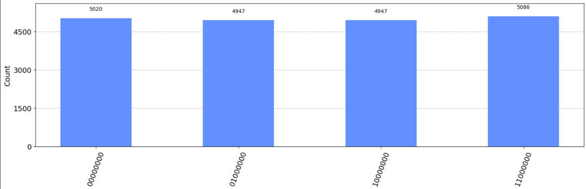
00000000, 01000000, 10000000, 11000000 それぞれの確率がほぼ等確率で得られたので、位相推定の結果は、

# 位相推定の結果
n = 8 # 位相推定用のビット数

estimated_thetas = [] # 推定された位相のリスト
for key, val in shor_qpe_counts.items():
    dec = 0 # 10進数の値
    for i, c in enumerate(key[::-1]):
        dec += (2**i)*int(c)
    estimated_theta = dec/(2**n)
    estimated_thetas.append(estimated_theta)

estimated_thetas.sort()
print(estimated_thetas)

[0.0, 0.25, 0.5, 0.75]

0.0, 0.25, 0.5, 0.75 のどれかという結果が得られた。

ex8

PythonのFractionライブラリを使って、位相推定した結果をs/rという分数で表現せよという問題。今回mod15なのでrは15未満。

from fractions import Fraction
shor_qpe_fractions = []# create a list of Fraction objects for each measurement outcome
for estimated_theta in estimated_thetas:
    shor_qpe_fractions.append(Fraction(estimated_theta).limit_denominator(15))

[Fraction(0, 1), Fraction(1, 4), Fraction(1, 2), Fraction(3, 4)]

ex9

いよいよショアのアルゴリズム全体を実装せよという問題。今まで使った関数やQPEを使えば実装できる。

ショアのアルゴリズムの回路や全体像は素因数分解アルゴリズムを学習する — 量子コンピューティング・ワークブックがわかりやすかったので、それを参考にして実装した。

ショアのアルゴリズムのフローチャート（量子コンピューティング・ワークブックから引用）。適切なrを求めるまで繰り返す

今回は7mod15ゲートのみを使うので、a=7で固定とする。

グレーダーにバグがあるっぽく、以下を実行してアップデートしたあと、カーネルを再起動する必要がある。

!pip install git+https://github.com/qiskit-community/Quantum-Challenge-Grader.git@main

"""ショアのQPE回路を作成する"""
def shor_qpe_circuit():
    phase_register_size = 8
    sys_register_size = 4
    shor_register_size = phase_register_size + sys_register_size

    shor_qpe = QuantumCircuit(shor_register_size, phase_register_size) #Create the QuantumCircuit needed to run with 8 phase register qubits

    # Step1: Preparation
    for i in range(phase_register_size):
        shor_qpe.h(i)
    shor_qpe.x(phase_register_size)

    # Step2: Apply cU
    for i in range(phase_register_size):
        cu = cU_multi(i)
        shor_qpe.append(cu, [i, *[phase_register_size+j for j in range(sys_register_size)]])

    # Spte3: Apply inversed-QFT    
    shor_qpe = qft_dagger(shor_qpe, phase_register_size)

    # Step4: Measure phase_register
    for i in range(phase_register_size):
        shor_qpe.measure(i, i)
    
    return shor_qpe

"""位相推定の結果を返す"""
def calc_estimated_phases(shor_qpe_counts):
    n = 8 # 位相推定用のビット数

    estimated_thetas = [] # 推定した位相のリスト
    for key, val in shor_qpe_counts.items():
        dec = 0 # 10進数の値
        for i, c in enumerate(key[::-1]):
            dec += (2**i)*int(c)
        estimated_theta = dec/(2**n)
        estimated_thetas.append(estimated_theta)

    # estimated_thetas.sort()
    return estimated_thetas

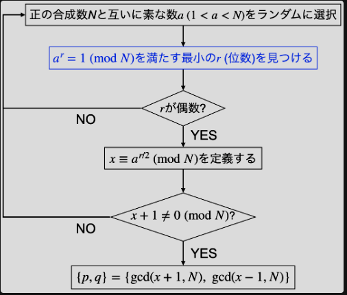
def shor_qpe(k):

    a = 7
    N = 15
    #Step 1. Begin a while loop until a nontrivial guess is found
    ### Your code goes here ###
    trivial_r = set() # だめだったrを保存しておく
    cnt = 0 # ループ回数
    while 1:
        cnt += 1
        if cnt == 20:
            # 無限ループを回避したい(20回やって駄目なら失敗とする)
            print("Not Found!!!!")
            break
        
        #Step 2a. Construct a QPE circuit with m phase count qubits
        #  to guess the phase phi = s/r using the function cU_multi()
        ### Your code goes here ###
        qpe_qc = shor_qpe_circuit()

        #Step 2b. Run the QPE circuit with a single shot, record the results
        # and convert the estimated phase bitstring to decimal
        ### Your code goes here ###
        sim = Aer.get_backend('aer_simulator')
        shots = 1 # シングルショットなので結果は1個だけなことに注意
        shor_qpe_counts = execute(qpe_qc, sim, shots=shots).result().get_counts()
        estimated_phases = calc_estimated_phases(shor_qpe_counts)

        #Step 3. Use the Fraction object to find the guess for r
        ### Your code goes here ###
        shor_qpe_fraction = Fraction(estimated_phases[0]).limit_denominator(15)
        r = shor_qpe_fraction.denominator
        if r in trivial_r:
            continue
        trivial_r.add(r)
            
        #Step 4. Now that r has been found, use the builtin greatest common deonominator
        # function to determine the guesses for a factor of N
        guesses = [gcd(a**(r//2)-1, N), gcd(a**(r//2)+1, N)]

        #Step 5. For each guess in guesses, check if at least one is a non-trivial factor
        # i.e.  (guess != 1 or N) and (N % guess == 0)
        ### Your code goes here ###
        is_ok = True
        for guess in guesses:
            if guess==1 or guess==N or N%guess!= 0:
                is_ok = False
        if guesses[0]*guesses[1] != N:
            is_ok = False
        if is_ok:
            break
    
    #Step 6. If a nontrivial factor is found return the list 'guesses', otherwise
    # continue the while loop
    ### Your code goes here ###
    print("ループ回数:", cnt)
    return guesses

実行結果。

m = 4
guesses = shor_qpe(m)
print(guesses)

ループ回数: 2
[3, 5]

（結構グレーダーゆるゆるで、N=15の素因数分解の答えとして[15, 1]を返すような関数でもパスした）

ベスパリブ

プログラミングを主とした日記・備忘録です。ベスパ持ってないです。

Qiskit Global Summer School 2023 Lab3 参加記録

各Labの記録

まえがき

Lab 3 : Diving Into Quantum Algorithms

ex1

ex2

ex3

ex4

ex5

ex6

ex7

ex8

ex9