はじめに

2022/11/11 ~ 11/18 の期間に開催された IBM Quantum Challenge Fall 2022 のメモ兼参加記録です。

内容としては以下のとおり。

Lab1: Qiskit Runtime、Sampler、Estimator入門
Lab2: Sampler、Estimatorの練習問題。量子サポートベクターマシンQSVMのお気持ち
Lab3: 組み合わせ最適化問題である巡回セールスマン問題のQUBO変換
Lab4: 量子化学計算VQE

lab1

Exercise 1

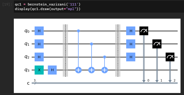
文字列 string が与えられたときのベルンシュタイン・ヴァジラニ回路の関数を作る。

def bernstein_vazirani(string):
    
    # Save the length of string
    string_length = len(string)
    
    # Make a quantum circuit
    qc = QuantumCircuit(string_length+1, string_length)
    
    # Initialize each input qubit to apply a Hadamard gate and output qubit to |->
    for i in range(string_length):
        qc.h(i)
    qc.x(string_length)
    qc.h(string_length)
    qc.barrier()
    
    # Apply an oracle for the given string
    # Note: In Qiskit, numbers are assigned to the bits in a string from right to left
    rev_string = string[::-1]
    for i in range(string_length):
        if rev_string[i] == "1":
            qc.cx(i, string_length)
    qc.barrier()
        
    # Apply Hadamard gates after querying the oracle
    for i in range(string_length):
        qc.h(i)
    
    # Measurement
    qc.measure(range(string_length), range(string_length))
    
    return qc

実行結果は以下のような感じ。

Exercise 2

回路qcは以下の形で与えられている。

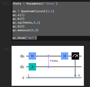
パラメータ theta に与える個々の位相 individual_phases も以下の形で与えられている。

phases = np.linspace(0, 2*np.pi, 50) # Specify the range of parameters to look within 0 to 2pi with 50 different phases

# Phases need to be expressed as list of lists in order to work
individual_phases = [[ph] for ph in phases]

Sampler を使い、パラメータ化された回路にパラメータをバインドする。以下が答え。

with Session(service=service, backend=backend):    
    sampler = Sampler(options=options)
    job = sampler.run(circuits=[qc for _ in range(50)], parameter_values=individual_phases)
    result = job.result()

上記のコードは、theta でパラメータ化された回路に、individual_phases の各パラメータをバインドしている。その50個分の回路の結果を実行し、集約された結果が得られるというわけらしい。

Exercise 3

【ステップ1】 RealAmplitudes を使ってランダムな回路を作る。

RealAmplitudes

# Make three random circuits using RealAmplitudes

n_qubit = 5
reps1 = 2
reps2 = 3
reps3 = 4

psi1 = RealAmplitudes(n_qubit, reps=reps1)
psi2 = RealAmplitudes(n_qubit, reps=reps2)
psi3 = RealAmplitudes(n_qubit, reps=reps3)

【ステップ2】 SparsePauliOp を使ってハミルトニアンを作る。

SparsePauliOpの使い方
- SparsePauliOp
- qiskit.quantum_info.SparsePauliOp.from_list

# Make hamiltonians using SparsePauliOp

H1 = SparsePauliOp.from_list([("IIZXI",1), ("YIIIY",3)])
H2 = SparsePauliOp.from_list([("IXIII",2)])
H3 = SparsePauliOp.from_list([("IIYII",3), ("IXIZI",5)])

【ステップ3】 numpy.linspace を使って theta の値を等間隔に作る。

# Make a list of evenly spaced values for theta between 0 and 1

theta1 = np.linspace(0, 1, n_qubit*(reps1+1))
theta2 = np.linspace(0, 1, n_qubit*(reps2+1))
theta3 = np.linspace(0, 1, n_qubit*(reps3+1))

【ステップ4】 Estimator を使って各期待値を計算する。

Estimatorの使い方
- Estimator
- qiskit.primitives.Estimator.run

# Use the Estimator to calculate each expectation value

with Session(service=service, backend=backend):
    
    options = Options(simulator={"seed_simulator": 42},resilience_level=0) # Do not change values in simulator
    
    estimator = Estimator(options=options)
        
    # calculate [ <psi1(theta1)|H1|psi1(theta1)>,
    #             <psi2(theta2)|H2|psi2(theta2)>,
    #             <psi3(theta3)|H3|psi3(theta3)> ]
    # Note: Please keep the order
    qcs = [psi1, psi2, psi3]
    pvs = [theta1, theta2, theta3]
    obs = [H1, H2, H3]
    job = estimator.run(circuits=qcs, parameter_values=pvs, observables=obs)

    result = job.result()

print(result)
# EstimatorResult(values=array([ 0.003 ,  1.749 , -1.0685]), metadata=[{'variance': 9.999775, 'shots': 4000}, {'variance': 0.9409989999999997, 'shots': 4000}, {'variance': 33.04502775, 'shots': 4000}])

Exercise 4

完全な誤り訂正符号の実装はオーバーヘッドがでかい。
このオーバーヘッドは現状、現実的ではない。
現時点では、小さなオーバーヘッドの実装で、エラー軽減することを目指している。
これらの技術はエラー緩和、エラー抑制と呼ばれている（関連するIBMの記事）。

Qiskit Runtimeには、よく使うエラー緩和とエラー抑制機能が組み込まれている。

DynamicalDecoupling
Sampler では、resilience_level=1 にするとM3が有効になる。
Estimator では、resilience_level=1 にするとT-REX、resilience_level=2 にするとデジタルZNEが有効になる。ほかにもエラー緩和策を選べる。

以下は、トリビア問題の回答。ほとんどテキストに書いてある。私の理解に沿った理由を記載するが、誤っている可能性があるので参考程度に。

誤り訂正は誤り軽減と同じである。
- 誤り。完全な誤り訂正の代替案として、エラー緩和やエラー抑制といった誤り軽減を利用している。
DDのためにX-gateを適用する場合、2回だけ適用することが可能である。
- 誤り。X-gateを2回適用するとなにもしないのと同じになるので、DDのためにこれをすることはある。が、2の倍数ならOKだろう。
DDには最適なデカップリング順序が重要である。
- 正しい。ハードウェアの都合上、パルスの長さは有限であり、完全な回転を実現できないので、適切なDDシーケンスを使用する必要がある。
M3 は量子測定誤差緩和のためのものである。
- 正しい。「M3は、スケーラブルな量子測定誤差軽減のためのパッケージで、割り当て行列やその逆行列を明示的に形成する必要がないため、行列不要の測定誤差軽減（matrix-free measurement mitigation, M3）ルーチンとなっています。（テキストの原文ママ）」
M3を使用する場合，Resilience levelを2に設定する必要がある。
- 誤り。Sampler では、resilience_level=1 にするとM3が有効になる。
T-REXはコヒーレントな誤差を確率的な誤差に変化させる。
- 正しい。「パウリ・トワリング」と呼ばれる手法でコヒーレントな誤差を確率的な誤差に変換している。
ZNEは誤り訂正技術であり、耐故障性QCに使用される。
- 誤り。誤り軽減技術である。
ZNEはノイズのスケールファクターを増幅し、ノイズがないときの測定値を推定する。
- 正しい。「ゼロノイズ外装(Digital Zero-noise Extrapolation, ZNE) を利用し、異なるノイズファクターに対する測定の期待値を計算し（増幅ステージ）、次に測定した期待値を使ってゼロノイズ限界での理想的な期待値を推測します（外挿ステージ）。この方法は期待値の誤差を減らす傾向がありますが、バイアスのない結果が得られることは保証されていません。（テキストの原文ママ）」
グローバル・フォールディングは、量子パルスを物理的に引き伸ばすアナログ的な方法である。
- 誤り。ローカル・フォールディングと同じ操作を回路全体に適用する、デジタル的な手法である。
ZNEを用いると、すべての誤差を軽減することができる。
- 誤り。期待値の誤差を減らす傾向はあるが、バイアスのない結果が得られるとは限らない。

Exercise 5

Sampler の回路は以下。

# build your code here
sampler_circuit = bernstein_vazirani("11111")

sampler_circuit.draw()

Estimator の回路は以下。

estimator_circuit = QuantumCircuit(2)

estimator_circuit.h(0)
estimator_circuit.cx(0,1)
estimator_circuit.ry(Parameter("theta"), 0)

estimator_circuit.draw()

各パラメータ、観測値は以下。

# parameters for estimator_circuit

number_of_phases = 10
phases = np.linspace(0, 2*np.pi, number_of_phases)
individual_phases = [[ph] for ph in phases]

# observables for estimator_circuit

Z0Z1 = SparsePauliOp.from_list([("ZZ",1)])
X0Z1 = SparsePauliOp.from_list([("ZX",1)])
Z0X1 = SparsePauliOp.from_list([("XZ",1)])
X0X1 = SparsePauliOp.from_list([("XX",1)])

ops = [Z0Z1, X0Z1, Z0X1, X0X1] # DO NOT CHANGE THE ORDER

Options の設定は以下。

# Import FakeBackend
fake_backend = FakeManila()
noise_model = NoiseModel.from_backend(fake_backend)

options_with_em = Options(
    simulator={ # Do not change values in simulator
        "noise_model": noise_model,
        "seed_simulator": 42,
    },
    # build your code here. Activate TREX for Estimator and M3 for sampler.
    resilience_level=1
)

以上の設定で、Sampler と Estimator を実行する。

with Session(service=service, backend=backend):
    
    sampler = Sampler(options=options_with_em)
    sampler_result = sampler.run(circuits=sampler_circuit).result()
    
    estimator = Estimator(options=options_with_em)
    estimator_result = []
    for op in ops:
        job = estimator.run(circuits=[estimator_circuit]*number_of_phases, parameter_values=individual_phases, observables=[op]*number_of_phases)
        result = job.result()
        estimator_result.append(result)

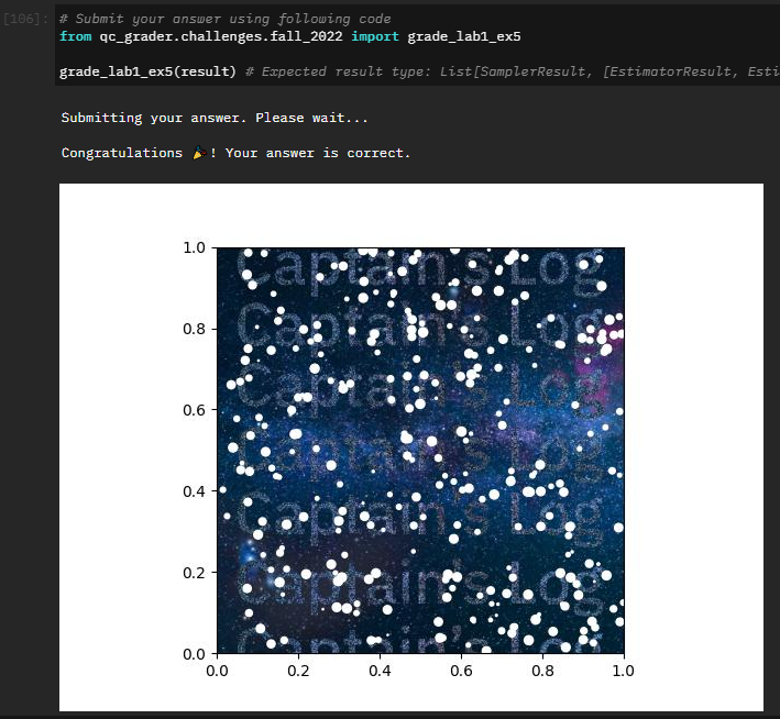
Exercise 6

message = "Captain's Log"

クリアすると限定公開の動画が見れる。今回、SFのストーリーがあり、しかも結構面白い。

Lab2

パラメータ化された量子回路

Exercise 1

from qiskit.circuit.library import RealAmplitudes

def lab2_ex1():
    qc = RealAmplitudes(num_qubits=4, reps=1, entanglement=[[0,1], [2,3], [1,2]], insert_barriers=True)
    
    return qc

qc = lab2_ex1()
qc.decompose().draw('mpl')

Exercise 2

M3について正誤問題。Lab1の4.1章を復習する。

Matrix-free Measurement Mitigation (M3) に関する以下の記述について、正しいか否かを答えてください。

Q1：M3は量子ゲートエラー緩和技術であり、フォールト・トレラントな量子コンピューターに使用される。
- 誤り。量子ゲートではなく、量子測定の誤差軽減技術である。
Q2：M3は、指数関数的なオーバーヘッドをランダムビット列の数によるスケーリングに落とし込んで作られる部分空間において動作する。
- 誤り。ランダムビット列ではなく、ノイズの多い入力ビット列によってスケーリングする。
Q3: M3は、ノイズのスケールファクターを増幅し、ノイズがない場合の測定値を推定する。
- 誤り。ゼロノイズ外挿（ZNE）の説明。
Q4: M3の技術は、直接的な解決方法と比較して、緩和のためのメモリー使用量を削減することができる。
- 正しい。行列を圧縮するので、メモリ使用量を削減できる。一般化最小残差法などを使った行列なしの方法もあるらしい。

Exercise 3

Sampler の文法がわかってきた。統計で例えると、回路のパラメータの個数が標本サイズで、sampler.run() で反復回数（標本数）だけ繰り返し実行するイメージ。

# 標本数 = n
theta_list = [[標本1], [標本2], ..., [標本n]]
sampler.run(circuits=[qc]*(標本数), parameter_values=theta_list, shots=shots)

で、以下が答え。

# create sampler using simulator and sample fidelities
with Session(service=service, backend=backend):
    sampler = Sampler(options=options)
    job = sampler.run(circuits=[fidelity_circuit]*len(theta_list), parameter_values=theta_list, shots=shots)
    fidelity_samples_sim = job.result()

    sampler = Sampler(options=options_noise)
    job = sampler.run(circuits=[fidelity_circuit]*len(theta_list), parameter_values=theta_list, shots=shots)
    fidelity_samples_noise = job.result()
    
    sampler = Sampler(options=options_with_em)
    job = sampler.run(circuits=[fidelity_circuit]*len(theta_list), parameter_values=theta_list, shots=shots)
    fidelity_samples_with_em = job.result()
    
fidelities_sim = []
fidelities_noise = []
fidelities_with_em = []

for i in range(10):
    fidelities_sim += [fidelity_samples_sim.quasi_dists[i][0]]
    fidelities_noise += [fidelity_samples_noise.quasi_dists[i][0]]
    fidelities_with_em += [fidelity_samples_with_em.quasi_dists[i][0]]

Exercise 4

ここ難しかった。

sample_train を使えと言われている。作成したいカーネル行列は対称な正方行列であるので……。

with Session(service=service, backend=backend):
    circuits = [fidelity_circuit]*circuit_num
    pvs = data_append(n, sample_train, sample_train)
    #
    sampler = Sampler(options=options_with_em)
    job =  sampler.run(circuits=circuits, parameter_values=pvs, shots=shots)
    quantum_kernel_em = job.result()
    #

Exercise 5

今回のカーネル行列は対称行列でないので、すべての要素を計算する必要がある。

たとえば行列の行をsample_train、列を未知のビット列に割り当てるとすると、行列の要素数は以下の通り。

n1 = len(unknown_data) # the number of unknown bit-string
n2 = 25 # the number of trained data
circuit_num_ex5 = n1*n2
print(circuit_num_ex5)

量子カーネル関数にデータをエンコードする関数は以下の通り。

def data_append_ex5(n1, n2, x1, x2):
    para_data_ex5 = []
    
    for i in range(n1):
        for j in range(n2):
            para_data_ex5.append(list(x1[i]) + list(x2[j]))
    
    return para_data_ex5

unknown_data と sample_train で計算されたカーネル行列：kernel_ex5 を計算するための Sampler のコードは以下の通り。

with Session(service=service, backend=backend):
    circuits_ex5 = [fidelity_circuit]*circuit_num_ex5
    pvs_ex5 = data_append_ex5(n1, n2, unknown_data, sample_train)
    
    sampler = Sampler(options=options_with_em)
    job =  sampler.run(circuits=circuits_ex5, parameter_values=pvs_ex5, shots=shots)
    quantum_kernel_ex5 = job.result()

Lab3

Exercise 1

qubit の数は、イジングモデルをイメージする。

# Let us first generate a graph with 4 nodes!

#### enter your code below ####

n = 4
num_qubits = n**2

#### enter your code above ####

tsp = Tsp.create_random_instance(n, seed=123)
adj_matrix = nx.to_numpy_matrix(tsp.graph)
print("distance\n", adj_matrix)

colors = ["r" for node in tsp.graph.nodes]
pos = [tsp.graph.nodes[node]["pos"] for node in tsp.graph.nodes]
draw_graph(tsp.graph, colors, pos)

Exercise2

与えられた二次問題をQUBOに変換し、イジングハミルトニアンを求めよという問題。

from qiskit_optimization.converters import QuadraticProgramToQubo

#### enter your code below ####

qp2qubo = QuadraticProgramToQubo()   #instatiate qp to qubo class
qubo = qp2qubo.convert(qp)      # convert quadratic program to qubo
qubitOp, offset = qubo.to_ising()      #convert qubo to ising

#### enter your code above ####

print("Offset:", offset)
print("Ising Hamiltonian:", str(qubitOp))

Exercise 3

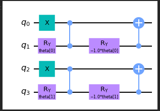
Matsuo, A., Suzuki, Y., & Yamashita, S. (2020). Problem-specific parameterized quantum circuits of the VQE algorithm for optimization problems. arXiv preprint arXiv:2006.05643.の論文の3.2.1節を参考にして、3量子ビットのW状態を構築せよという問題。

from qiskit import QuantumRegister, ClassicalRegister
from qiskit.circuit import ParameterVector, QuantumCircuit

# Initialize circuit
qr = QuantumRegister(3)
cr = ClassicalRegister(3)
circuit = QuantumCircuit(qr,cr)

# Initialize Parameter with θ
theta = ParameterVector('θ', 2)

#### enter your code below ####

# Apply gates to circuit
circuit.x(0)
circuit.ry(theta[0], 1)
circuit.cz(0,1)
circuit.ry(-theta[0], 1)
circuit.ry(theta[1], 2)
circuit.cz(1,2)
circuit.ry(-theta[1], 2)
circuit.cx(1,0)
circuit.cx(2,1)

#### enter your code above ####

circuit.measure(qr,cr)
circuit.draw("mpl")

Exercise 4

from qiskit_ibm_runtime import Session, Sampler, Options

options = Options(simulator={"seed_simulator": 42},resilience_level=0) #DO NOT CHANGE

#### Enter your code below ####

# Define sampler object
with Session(service=service, backend=backend):
    pvs = [[(54.73/360)*(2*np.pi), (45/360)*(2*np.pi)]] 
    
    sampler = Sampler(options=options) # Define sampler with options above
    result = sampler.run(circuits=[circuit], parameter_values=pvs, shots=5000).result() # Run the sampler. Remember, the theta here is in degrees! :) 
    
# Plot result 
result_dict = result.quasi_dists[0] # Obtain the quasi distribution. Note: Expected result type: QuasiDistribution dict

#### Enter your code above ####

values = list(result_dict.keys()) # Obtain all the values in a list
probabilities = list(result_dict.values()) # Obtain all the probabilities in a list

plt.bar(values,probabilities,tick_label=values)
plt.show()
print(result_dict)

Exercise 5

N量子ビットのTSPエンタングラー・ルーチンを構築する関数を作成せよという問題。こういうの見るたび競プロやってて良かったと思う。

from qiskit import QuantumRegister, ClassicalRegister
from qiskit.circuit import ParameterVector, QuantumCircuit

def tsp_entangler(N):
    
    # Define QuantumCircuit and ParameterVector size
    circuit = QuantumCircuit(N**2)
    theta =  ParameterVector('theta',length=(N-1)*N)
    
    ############# 
    # Hint: One of the approaches that you can go for is having an outer `for` loop for each node and 2 inner loops for each block. /
    # Continue on by applying the same routine as we did above for each node with inner `for` loops for /
    # the ry-cz-ry routine and cx gates. Selecting which indices to apply for the routine will be the /
    # key thing to solve here. The indices will depend on which parameter index you are checking for and the current node! /
    # Reference solution has one outer loop for nodes and one inner loop each for rz-cz-ry and cx gates respectively.
    ############# 
    
    #### enter your code below ####
    theta_i = 0
    for i in range(N):
        # X Gate
        circuit.x(i*N)
    
        # Parameter Gates
        for j in range(i*N+1, i*N+N):
            circuit.ry(theta[theta_i], j)
            circuit.cz(j-1, j)
            circuit.ry(-theta[theta_i], j)
            theta_i += 1
        
        # CX gates
        for j in range(i*N+1, i*N+N):
            circuit.cx(j, j-1)
        
    #### enter your code above ####

    return circuit

Exercise 6

VQE
qiskit.algorithms.minimum_eigensolvers.MinimumEigensolver.compute_minimum_eigenvalue VQEはQuantum Primitive用にリファクタリングされたらしく、検索しても古い方法しか出てこない。テキストを読んでお気持ちエスパーしながら実装する。

引数:

estimator: ハミルトニアン演算子の期待値を計算するためのestimator primitive。

ansatz: 試行状態のためのパラメーター化された量子回路。

optimizer: 最小エネルギーを求めるための古典的なオプティマイザー。Qiskit.Optimizer、または.Minimizerプロトコルを実装したcallableとすることができる。

initial_point: オプティマイザーの初期点（つまり、パラメーターの初期値）。初期点の長さは、ansatzのパラメーターの数と一致しなければならない。Noneの場合、特定のパラメーター範囲内でランダムな点が生成されます。SamplingVQEは、この範囲をansatzから求めます。ansatzが範囲を指定していない場合、-2\pi, 2\piの範囲が使用されます。

callback: 各最適化ステップで中間データにアクセスできるコールバック。これらのデータは、評価回数、ansatzのオプティマイザーのパラメーター、estimatorの値、およびメタデーターの辞書です。

まず、3ノードのTSPエンタングラーを作成しておく。

# Define PQC for 3 node graph (Hint: Call the previous function you just made)
PQC = tsp_entangler(3)

RunVQE 関数は以下の通り。

def RunVQE(estimator, model, optimizer, operator, init=None):
    
    # Store intermediate results
    history = {"eval_count": [], "parameters": [], "mean": [], "metadata": []}
    
    # Define callback function
    def store_intermediate_result(eval_count, parameters, mean, metadata):
        history["eval_count"].append(eval_count)
        history["parameters"].append(parameters)
        history["mean"].append(mean.real)
            
    #### Enter your code below ####
    
    # Define VQE run
    vqe = VQE(estimator=estimator, ansatz=model, optimizer=optimizer, initial_point=init, callback=store_intermediate_result)

    # Compute minimum_eigenvalue
    result = vqe.compute_minimum_eigenvalue(operator=operator, aux_operators=None)
    
    #### Enter your code above ####

    return result, history["mean"]

VQEを実行し、結果を得るためのコードは以下の通り。Estimator に options を渡さないことに注意。

%%time
# Do not change the code below and use the given seeds for successful grading
from qiskit.utils import algorithm_globals
from qiskit.primitives import Estimator
algorithm_globals.random_seed = 123

# Define optimizer
optimizer = SPSA(maxiter=50)

# Define Initial point
np.random.seed(10)
init = np.random.rand((n-1)*n) * 2 * np.pi

# Define backend
backend = service.backends(simulator=True)[0]

#### Enter your code below ####

# Call RunVQE
with Session(service = service, backend = backend):
    estimator = Estimator()
    result, mean = RunVQE(estimator=estimator, model=PQC, optimizer=optimizer, operator=qubitOp, init=init) #----# Enter your code here. Do not pass in options)
        
#### Enter your code above ####

# Print result
print(result)

Exercise 7

前回計算したVQE結果から得られたパラメータを使って、最適化回路に渡す。

テキストに書いてあるが、Estimator に渡す parameter_values 引数は、result.optimal_parameters の値を渡す。

def BestBitstring(result, optimal_circuit):
    energy = result.eigenvalue.real
    
    options = Options(simulator={"seed_simulator": 42},resilience_level=0) # Do not change and please pass it in the Sampler call for successful grading
    
    #### enter your code below ####
    with Session(service = service, backend = backend):
        # Enter your code here. Please do pass in options in the Sampler construct.
        sampler = Sampler(options=options)
        job = sampler.run(circuits=[optimal_circuit], parameter_values=[list(result.optimal_parameters.values())])
        sampler_result = job.result() 

    # Obtain the nearest_probability_distribution for the sampler result from the quasi distribution obtained
    result_prob_dist = sampler_result.quasi_dists[0].nearest_probability_distribution()
   
    #### enter your code above ####
    
    max_key = format(max(result_prob_dist, key = result_prob_dist.get),"016b")

    result_bitstring = np.array(list(map(int, max_key)))
    
    return energy, sampler_result, result_prob_dist, result_bitstring

Exercise 8

一般化よくわかんなかったです👽。

n = 3
model_3 = QuantumCircuit(n**2)
theta = ParameterVector('theta',length=(n-1)*n//2)

# Build a circuit when n is 2
model_3.x(0)
model_3.x(6)

# Apply a parameterized W state gate
model_3.ry(theta[0],1)
model_3.cz(0,1)
model_3.ry(-theta[0],1)
model_3.cx(1,0)
model_3.cx(1,3)
model_3.cx(0,4)

model_3.ry(theta[1],7)
model_3.cz(6,7)
model_3.ry(-theta[1],7)

model_3.ry(theta[2],8)
model_3.cz(7,8)
model_3.ry(-theta[2],8)

model_3.cx(7,6)
model_3.cx(8,7)

# Apply 4 CSWAP gates
model_3.cswap(6,0,2)
model_3.cswap(6,5,3)
model_3.cswap(7,1,2)
model_3.cswap(7,4,5)

model_3.draw("mpl")

Exercise 9

4ノードでVQE解を求めよという問題。いままで作った関数を駆使して実装する。

QUBO は以下の通り。

#### Enter your code below ####

qp = tsp.to_quadratic_program()
qp2qubo = QuadraticProgramToQubo()
qubo = qp2qubo.convert(qp)
qubitOp_4, _ = qubo.to_ising()

#### Enter your code above ####

model は以下の通り。なんかソラから実装させようとしてきたけど、めんどくさいのでしない。

model = tsp_entangler(n)

Lab4

化学わかんね～～～🧪🤷

Exercise 1

Å ：オングストロームと読む。1Å = 10^{-10} メートル。

value の値は、図の「？？？」の距離を計算する。正三角形なので計算できるのだが、小数点第6位まできっかりの値じゃないと grade はクリアできない。どういうこと？

Molecule モジュールのページが Not Found なのでエスパーすると、

hydrogen_t = [["原子記号", [x座標, y座標, z座標]], ...]
multiplicity は、多重度。今回は1らしい（テキストに書いてある）。
charge は、電荷？たぶん1。

#### Fill in the values below and complete the function to define the Molecule ####

# Coordinates are given in Angstrom
# value = 0.791513 / 3**(1/2)  # 0.4569802436170883
value = 0.456980
hydrogen_t = [["H", [value, 0.0, 0.0]], # ----------- Enter your code here
              ["H", [-value, 0.0, 0.0]], # ----------- Enter your code here
              ["H", [0.0, 0.791513, 0.0]]]
                  
h3p = Molecule( # Fill up the function below
    geometry=hydrogen_t, # ----------- Enter your code here
    multiplicity=1, # ----------- Enter your code here
    charge=1, # ----------- Enter your code here
)

driver = ElectronicStructureMoleculeDriver(h3p, basis="ccpvdz", driver_type=ElectronicStructureDriverType.PYSCF) 

properties = driver.run()

Exercise 2

次に、Estimator を使ってどのようにルーチンを設定するかを定義します。Estimatorは量子回路から推定される期待値と物理量を返します。ここで渡す回路は私たちの ansatz で、物理量は先ほど作成した qubit_op_parity ハミルトニアンで、パラメータ値はここで x として渡した古典オプティマイザーで処理される値です。この例では、同時摂動確率的近似(SPSA)オプティマイザーを使用しています。（テキスト引用）

optimizer で最小化するスカラー関数は evaluate_expectation 。x0 引数には initial_point を入れる。

サンプルコード内の job_list には、PrimitiveJob ではなく実際には EstimatorResult が入る。ややこしい。

%%time
from qiskit.utils import algorithm_globals
algorithm_globals.random_seed = 1024

# Define convergence list
convergence = []

# Keep track of jobs (Do-not-modify)
job_list = []

# Initialize estimator object
estimator = Estimator()# Enter your code here

# Define evaluate_expectation function
def evaluate_expectation(x):
    x = list(x)
    
    # Define estimator run parameters
    #### enter your code below ####
    # job = estimator.run(circuits=[ansatz], observables=[qubit_op_parity], parameter_values=[x]) # PrimitiveJob ではなく、EstimatorResultを入れる
    job = estimator.run(circuits=[ansatz], observables=[qubit_op_parity], parameter_values=[x]).result() # ----------- Enter your code here
    results = job.values[0]
    job_list.append(job)
    
    # Pass results back to callback function
    return np.real(results)

# Call back function
def callback(x,fx,ax,tx,nx):
    # Callback function to get a view on internal states and statistics of the optimizer for visualization
    convergence.append(evaluate_expectation(fx))

np.random.seed(10)

# Define initial point. We shall define a random point here based on the number of parameters in our ansatz
initial_point = np.random.random(ansatz.num_parameters)

#### enter your code below ####
# Define optimizer and pass callback function
optimizer = SPSA(maxiter=50, callback=callback) # ----------- Enter your code here

# Define minimize function
result = optimizer.minimize(fun=evaluate_expectation, x0=initial_point) # ----------- Enter your code here

Exercise 3

construct_problem は以下。

def construct_problem(geometry, charge, multiplicity, basis, num_electrons, num_molecular_orbitals):

    molecule = Molecule(geometry=geometry,
                            charge=charge, 
                            multiplicity=multiplicity) 
    driver = ElectronicStructureMoleculeDriver(molecule, basis=basis, driver_type=ElectronicStructureDriverType.PYSCF) 

    # Run the preliminary quantum chemistry calculation
    properties = driver.run()

    # Set the active space
    active_space_trafo = ActiveSpaceTransformer(num_electrons=num_electrons,
                                        num_molecular_orbitals=num_molecular_orbitals) 

    # Now you can get the reduced electronic structure problem
    problem_reduced = ElectronicStructureProblem(driver, transformers=[active_space_trafo]) # ----------- Enter your code here

    # The second quantized Hamiltonian of the reduce problem
    second_q_ops_reduced = problem_reduced.second_q_ops()

    # Set the mapper to qubits
    parity_mapper = ParityMapper() # This is the example of parity mapping

    # Set the qubit converter with two qubit reduction to reduce the computational cost 
    parity_converter = QubitConverter(parity_mapper) # ----------- Enter your code here    

    # Compute the Hamitonian in qubit form
    qubit_op_parity = parity_converter.convert(second_q_ops_reduced.get('ElectronicEnergy'), num_particles=problem_reduced.num_particles)
   
    # Get reference solution
    vqe_factory = VQEUCCFactory(quantum_instance=StatevectorSimulator(),optimizer=SLSQP(),ansatz=UCC(excitations='sd')) 
    solver = GroundStateEigensolver(parity_converter, vqe_factory)    
    real_solution = solver.solve(problem_reduced).total_energies[0]    
    
    ansatz=vqe_factory.ansatz
    
    return ansatz, qubit_op_parity, real_solution, problem_reduced

custom_vqe は以下。

def custom_vqe(estimator, ansatz, ops, problem_reduced, optimizer = None, initial_point=None):

    # Define convergence list
    convergence = []

    # Keep track of jobs (Do-not-modify)
    job_list = []

    # Define evaluate_expectation function
    def evaluate_expectation(x):
        x = list(x)

        # Define estimator run parameters
        job = estimator.run(circuits=[ansatz], observables=[ops], parameter_values=[x]).result() # ----------- Enter your code here
        results = job.values[0]
        job_list.append(job)

        # Pass results back to callback function
        return np.real(results)

    # Call back function
    def callback(x,fx,ax,tx,nx):
        # Callback function to get a view on internal states and statistics of the optimizer for visualization
        convergence.append(evaluate_expectation(fx))

    np.random.seed(10)

    # Define initial point. We shall define a random point here based on the number of parameters in our ansatz
    if initial_point is None:
        initial_point = np.random.random(ansatz.num_parameters)

    # Define optimizer and pass callback function
    if optimizer == None:
        optimizer = SPSA(maxiter=50, callback=callback)

    # Define minimize function
    result = optimizer.minimize(fun=evaluate_expectation, x0=initial_point) # ----------- Enter your code here

    vqe_interpret = []
    for i in range(len(convergence)):
        sol = MinimumEigensolverResult()
        sol.eigenvalue = convergence[i]
        sol = problem_reduced.interpret(sol).total_energies[0]
        vqe_interpret.append(sol)

    return vqe_interpret, job_list, result

grade_lab4_ex3b は、grade_lab4_ex に修正する。

## Grade and submit your solution
from qc_grader.challenges.fall_2022 import grade_lab4_ex3

grade_lab4_ex3(construct_problem, custom_vqe)

Exercise 4

construct_problem で電子構造問題を作成する。
custom_vqe で基底状態エネルギーを計算する。
グラフ化する。

という流れ。

反応エネルギーを単位[eV]で求めよという問題。

反応エネルギー = 反応後のエネルギー - 反応前のエネルギー

VQE実行の最終的な収束値を使って計算すれば良い。

K_H2eV = 27.2113845  # Hartree -> eV

# calculate reaction energy.
before_energy = (Energy_H_m[-1] + Energy_H_c[-1])
after_energy = (Energy_H_t[-1] + Energy_H_a[-1])
react_energy = after_energy - before_energy

react_vqe_ev = react_energy * K_H2eV # Fill this cell. Please note the reaction energy should be in eV and not in Hartree units for succesful grading.

print("Reaction energy VQE estimator eV", react_vqe_ev ,"\n")

Exercise 5

Variational Quantum Deflation (VQD) ルーチンを用いた第一励起状態遷移エネルギー（nm単位）を求める問題。

%%time
# Extracting solved initial point from one shot estimation done previously
initial_pt = result.raw_result.optimal_point

# List to store all estimated observables
uccsd_result = [] 

#### Enter your code below ####
for i in range(7):
    uccsd_result.append(Estimator().run(circuits=[vqe_factory.ansatz], observables=[qubit_op_parity[i]], parameter_values=[initial_pt]).result())
#### Enter your code above ####
        
energy_c_estimator=uccsd_result[0].values[0]+result.extracted_transformer_energy+result.nuclear_repulsion_energy

print('Energy =  ', energy_c_estimator)

シクロプロペニリデンの全双極子モーメントを求める問題。

双極子モーメントは、分極のベクトルの和であるらしい。方向（符号）に気をつけて足し合わせたあと、ベクトルのマグニチュードを求めれば良い。

双極子モーメント = 活性化双極子モーメント + トランスフォーマーによって抽出された双極子モーメント - 核双極子モーメント

# Fill your codes here, dipole moment computed by Nuclear dipole moment - Electronic dipole moment 
# and Electronic dipole moment computed by adding VQE reult and ctiveSpaceTransformer extracted energy part

dipxau = uccsd_result[4].values[0] + temp_dipoles[0] - temp_nu_dipoles[0] # ----------- Enter your code here (Use Partial information in element 4 in uccsd_result list)
dipyau = uccsd_result[5].values[0] + temp_dipoles[1] - temp_nu_dipoles[1] # ----------- Enter your code here (Use Partial information in element 5 in uccsd_result list)
dipzau = uccsd_result[6].values[0] + temp_dipoles[2] - temp_nu_dipoles[2] # ----------- Enter your code here (Use Partial information in element 6 in uccsd_result list)

au2debye =  1/0.393430307 # Convert to debye
dipxdebye = dipxau.real * au2debye
dipydebye = dipyau.real * au2debye
dipzdebye = dipzau.real * au2debye

dip_tot = (dipxdebye**2 + dipydebye**2 + dipzdebye**2)**(1/2) # Compute the total dipole moment magnitude here from the individual components of the vector computed above.
print('Dipole (debye) : ', dip_tot)

Final Ranked Exercise

ノイズのある回路でVQE実行するチャレンジ問題。

HACK TO THE FUTURE 2023 予選（AtCoder Heuristic Contest 016）と期間丸かぶりしてて時間なくてやってません＞＜

おわりに

今回はSFのストーリーがあって、ブラックホールからスイングバイ脱出するという目的のもと、スペースデブリの効率的な排除のために巡回セールスマン問題をQUBOを使って解いたり、燃料を節約するために宇宙空間の化学物質の分子特性をVQEを構築して計算するといった流れになっていた。演出もなかなか力が入っていて、ただ単に問題を解くよりもエンターテイメントって感じで面白かったです。

去年と同様、修了証明書としてのバッジをもらえました。

ベスパリブ

プログラミングを主とした日記・備忘録です。ベスパ持ってないです。

IBM Quantum Challenge Fall 2022 参加記録

はじめに

lab1

Exercise 1

Exercise 2

Exercise 3

Exercise 4

Exercise 5

Exercise 6

Lab2

Exercise 1

Exercise 2

Exercise 3

Exercise 4

Exercise 5

Lab3

Exercise 1

Exercise2

Exercise 3

Exercise 4

Exercise 5

Exercise 6

Exercise 7

Exercise 8

Exercise 9

Lab4

Exercise 1

Exercise 2

Exercise 3

Exercise 4

Exercise 5

Final Ranked Exercise

おわりに